Model Submissions for Ethereum Deep Funding

thedevanshmehta · May 16, 2025, 6:43am

Hello model builders,

Consider this thread as your home for sharing all things related to your submissions in the deep funding challenge giving weights to the Ethereum dependency graph

In order to be eligible for the $25,000 prize pool, you need to make a detailed write-up of model submissions. You may submit this even after September 7th 2025, once the deadline for the contest is over. However, it needs to be submitted by September 20th.

$10,000 is given objectively based on leaderboard placement while $10,000 is on quality of writeups here. $5000 is kept aside for the jury to evaluate and give feedback on your models.

We will give additional points to submissions with open source code and fully reproducible results. We encourage you to be visual in your submissions, share your jupyter notebooks or code used in the submission, explain the difference in performance of the same model on different parts of the ethereum graph and share information that is collectively valuable to other participants.

Since write-ups can be made after submissions close, other participants cannot copy your methodology. You can take cues for writeups from other competition we have held and also get some inspiration for baking your own model.

The format of submissions is open ended and free for you to express yourself the way you like. You can share as much or as little as you like, but you need to write something here to be considered for prizes.

More details at deepfunding.org

Good luck predictoooors

abbamaster0 · July 16, 2025, 9:33am

Quantifying Contributions of Open Source Projects to the Ethereum Universe

Overview

Ethereum, as a decentralized and rapidly evolving ecosystem, is built on the back of countless open-source projects. From core protocol implementations and smart contract frameworks to tooling, middleware, and developer libraries, the growth of the Ethereum universe is directly tied to the strength and progress of its open-source foundation.

Despite this, there is currently no widely adopted method to quantitatively evaluate the impact of individual open-source projects within Ethereum. This lack of visibility impairs the ability of stakeholders—including the Ethereum Foundation, DAOs, developers, researchers, and funders—to identify which projects are truly foundational and deserving of support, auditing, or recognition.

This initiative proposes a data-driven framework for quantifying the contributions of open-source repositories to Ethereum using a combination of ecosystem relevance, technical dependencies, development activity, and on-chain influence. The goal is to build a transparent, scalable, and objective system to rank the importance of repositories across the Ethereum universe.

Why Quantification Matters

Funding Allocation: Improve the accuracy and fairness of grants, retroactive public goods funding, and quadratic funding.

Ecosystem Security: Identify critical libraries and infrastructure projects that require audits and monitoring.

Developer Recognition: Highlight unsung contributors and undervalued repos with high ecosystem leverage.

Governance Insights: Support DAO tooling and decision-making with data-driven repository influence scores.

Sustainability: Ensure long-term viability of critical infrastructure by recognizing and supporting maintainers.

Core Evaluation Dimensions

To quantify contributions effectively, the model should evaluate repositories along multiple, weighted dimensions:

Development Activity

Commit frequency, pull requests, issue resolution

Contributor diversity and project longevity

Ecosystem Dependency

How many other repos depend on it (import graphs, dev toolchains)

Used in major L2s, DeFi protocols, wallets, or clients

On-Chain Impact

Smart contracts linked to repo deployed on-chain

Volume of interactions, transaction count, or TVL influenced

Protocol Alignment

Inclusion in Ethereum Improvement Proposals (EIPs)

Alignment with Ethereum’s roadmap (e.g., scalability, account abstraction, L2s)

Community Footprint

Mentions in dev discussions (e.g., EthResearch, Reddit, Twitter)

Citations in academic or technical Ethereum publications

Quantification Methodology

The proposed methodology involves:

Repository Indexing: Identify a comprehensive list (~15,000) of Ethereum-relevant open-source repositories.

Data Aggregation: Pull data from GitHub, The Graph, GHTorrent, npm, smart contract registries (e.g., Etherscan), and social platforms.

Metrics Standardization: Normalize and weight features across categories (e.g., activity, adoption, dependency).

Modeling: Use rule-based scoring or machine learning models (e.g., gradient boosting, GNNs) to compute a unified contribution score.

Result: A ranked list of repositories with associated weights reflecting their quantified contributions to Ethereum.

Output Example

go-ethereum: 0.98

solidity: 0.95

OpenZeppelin/contracts: 0.89

ethers.js: 0.86

foundry-rs/foundry: 0.82

Lido-finance/lido-dao: 0.74

Uniswap/v3-core: 0.72

eth-infinitism/account-abstraction: 0.67

Scores are illustrative

Potential Applications

Grant Program Optimization (EF, Gitcoin, ARB Grants)

Retroactive Airdrops and Rewards (e.g., Optimism RPGF)

Reputation Systems for Devs and DAOs

Ecosystem Risk Mapping

Dynamic Leaderboards and Dashboards

Challenges and Limitations

Attribution Complexity: Linking code to impact is non-trivial and may involve indirect relationships.

Gaming and Bias: Repos could be gamed through artificial commits or inflated usage.

Subjectivity in Weighting: Choosing the right weights across dimensions can influence final scores; requires transparency and community input.

Temporal Dynamics: Repo relevance changes over time and needs continuous updates.

ewohirojuso · July 21, 2025, 12:09pm

Project Background

I took on this contest to analyze the contribution of various code repositories within the Ethereum ecosystem. In essence, it involved scoring and ranking these repositories to determine their importance to the overall ecosystem. What seemed straightforward at first turned out to have quite a few hidden complexities.
My name is ewohirojuso and mail is ewohirojuso66@gmail.com

Overall Architecture

The entire system is divided into several core modules:

ArrayManager: Handles GPU acceleration.
FastCompute: For high-performance computations.
GraphConstructor: Builds dependency graphs.
TopologyFeatures: Extracts network topological features.
ImpactModel: Implements machine learning prediction models.
WeightEngine: Calculates weights.

The code structure is clear, with each module having a single responsibility. GPU acceleration was used primarily because of the large volume of data, which would be too slow to process on a standard CPU.

Design and Implementation of the Feature Standardization System

In this development, I believe the most valuable aspect to share is the feature standardization system. Initially, I didn’t give it much thought, assuming it was just basic data preprocessing. However, I soon discovered its surprising depth.

Problems Encountered

Vast differences in original data feature distributions: Some feature values ranged from 0-1 (e.g., win rate), while others were in the tens or hundreds of thousands (e.g., star count), and some were logarithmic (e.g., PageRank values). Feeding this raw data directly into the model resulted in abysmal performance.
Traditional Z-score standardization was not effective: Due to numerous outliers, traditional Z-score standardization didn’t work well here. For instance, a sudden surge in star count for a particular repository, acting as an outlier, would severely skew the entire distribution.

Solution

I implemented a robust standardization method based on the median and Interquartile Range (IQR):

def _initialize_feature_scalers(self) -> Dict[str, Dict[str, float]]:
    feature_statistics = defaultdict(list)
    
    # Collect all feature values
    for repo_features in self.all_features.values():
        for feature_name, value in repo_features.items():
            if not (pd.isna(value) or np.isinf(value)):
                feature_statistics[feature_name].append(float(value))
    
    scalers = {}
    for feature_name, values in feature_statistics.items():
        if len(values) > 0:
            values_array = np.array(values)
            scalers[feature_name] = {
                'median': np.median(values_array),
                'p75': np.percentile(values_array, 75),
                'p25': np.percentile(values_array, 25)
            }
    return scalers

The core idea is to replace the mean with the median and the standard deviation with the IQR:

def _standardize_feature_value(self, feature_name: str, value: float) -> float:
    if feature_name not in self.feature_scalers:
        return value
        
    scaler = self.feature_scalers[feature_name]
    
    median = scaler['median']
    iqr = scaler['p75'] - scaler['p25'] + 1e-8
    
    standardized = (value - median) / iqr
    
    # Soft clipping to avoid extreme outliers
    return np.tanh(standardized * 0.5) * 2.0

Why This Design?

Robustness: The median and IQR are insensitive to outliers and won’t be skewed by individual extreme values.
Soft Clipping: Using the tanh function for soft clipping limits the influence of extreme values while preserving their relative magnitudes.
Feature Type Adaptation: Different types of features are combined with different weighting strategies.

Actual Results

After switching to this standardization method, the model’s cross-validation score increased from just over 0.2 to over 0.4, a significant improvement. This was particularly effective for features with clear outliers, such as the star count of repositories.

Some Pitfalls Encountered

Division by Zero: IQR can be 0 (if all values are the same), so a small epsilon must be added to prevent division by zero.
Handling Missing Values: NaN and Inf values must be filtered out first, otherwise they will contaminate the statistics.
Feature Alignment: Ensure all repositories have the same set of features, filling in missing ones with default values.

# Tips for handling division by zero and missing values
iqr = scaler['p75'] - scaler['p25'] + 1e-8  # Prevent division by zero
standardized = (value - median) / iqr
return np.tanh(standardized * 0.5) * 2.0    # Limit to [-2,2] range

Other Technical Highlights

GPU Acceleration

We used CuPy for matrix operation acceleration, primarily during feature computation and model training. For large-scale network analysis, GPUs are indeed significantly faster than CPUs.

Machine Learning Model

Ultimately, XGBoost was chosen, mainly because it’s less demanding on feature engineering and has existing GPU support. Several other models were tried, but none performed as well as XGBoost.

Weight Allocation Strategy

This part is central to the entire system. We adopted a multi-level weight allocation approach: seed project weights, originality scores, and dependency relationship weights. Each layer has its unique calculation logic.

Throughout this project, the biggest takeaway was the critical importance of data preprocessing. Feature standardization might seem like a minor issue, but it profoundly impacts the final results. Often, poor model performance isn’t due to the algorithm itself, but rather how the data is fed into the model.

Furthermore, GPU acceleration is truly valuable, especially when dealing with large-scale graph data. However, careful memory management is crucial, as GPU memory is much more precious than CPU memory.

The code has been uploaded, and I welcome any discussions. This type of ecosystem analysis project is quite interesting, offering both engineering challenges and opportunities for algorithmic optimization.

summer · July 21, 2025, 3:29pm

Author: summer
renzhichua1@gmail.com
Version/Date: v2.12 / 2025-07-02

1. Data-Driven and Systematized Engineering

Facing the complex task of quantifying contributions to the Ethereum ecosystem, our core design philosophy is to build a robust, reproducible, and deeply data-driven systematized solution. We believe that excellent results do not just stem from a single clever algorithm, but rather rely on meticulously engineered design at every stage, from data processing and feature construction to model training and weight allocation.

Our solution aims to minimize reliance on hard-coded rules and subjective assumptions, instead building upon the following principles:

Maximize Data Utilization: We not only leverage raw training data but also extract implicit relationships from existing data through Data Augmentation techniques to enhance the model’s generalization ability.
Deep Feature Engineering: We believe that the quality of features directly determines the upper limit of model performance. Therefore, we have constructed a comprehensive system of multi-dimensional features, including network topology, team quality, historical performance, contributor profiles, and temporal evolution.
Layered Machine Learning: For the multi-level (Level 1, 2, 3) weight allocation tasks in the competition, we adopted different strategies. Notably, we elevated the Level 2 (originality) weight allocation, traditionally dependent on heuristic rules, into an independent machine learning task.

This report will focus on elaborating the key innovations in our scheme: machine learning modeling for Level 2 weights, and Enhanced Feature Representation for relation prediction.

2. Key Innovations: Layered Machine Learning and Enhanced Feature Representation

Our system features deep innovation in two key areas, aiming to replace fixed rules with learned patterns, thereby improving overall accuracy and robustness.

Machine Learning Modeling for Level 2 (Originality) Weights

“Originality” is a highly subjective concept. Traditional approaches typically rely on heuristic rules based on dependency count (e.g., more dependencies mean less originality). We believe this method is too crude and fails to capture complex realities.

To address this, we designed the ImprovedLevel2Allocator module, which transforms originality scoring itself into a supervised learning problem.

The key idea is: If a project frequently wins in direct comparisons with the libraries it depends on, this strongly indicates that it generates significant added value itself, i.e., it has high originality.

Our implementation steps are as follows:

Signal Extraction: We filter all direct comparison records between “parent projects” and their “child dependencies” from the training data. For example, when web3.py is compared to its dependency eth-abi, the result (win/loss and multiplier) becomes a strong signal for measuring web3.py’s originality.
Feature Construction: We build a set of feature vectors specifically for predicting originality for each core project (seed repo). Key features include:
- Win rate against dependencies (win_rate_against_deps): This is the most crucial metric, directly reflecting the project’s ability to surpass its underlying dependencies.
- Dependency count and depth (dependency_count, max_dependency_depth): Serve as basic penalty terms.
- Comprehensive quality metrics: Reusing features from the main feature library such as team quality, network influence, and historical performance.
Model Training: We use a GradientBoostingRegressor model, with these features as input and a “true” originality score (estimated by combining multiple signals) as the label, for model training. Cross-validation results show that the model’s R² score reached a respectable level, proving the feasibility of this approach.

Through this method, we upgraded the evaluation of originality from a simple “rule engine” to an “intelligent model” capable of learning complex patterns from data, whose judgments are far richer and more precise than simple dependency counting.

Enhanced Feature Representation and Data Augmentation for Relation Prediction

When predicting the relative contribution between two repositories (Repo A vs. Repo B), how effectively to present their differences to the model is crucial. Simply subtracting the feature vectors of the two repositories (feature_A - feature_B) loses a lot of scale and proportional information.

To address this, in AdvancedEnsemblePredictor, we designed the _create_enhanced_feature_vector function to generate a “feature group” for each original feature, containing multiple comparison methods:

Simple difference (A - B): Captures absolute differences.
Safe ratio (A / B): Captures relative proportions, crucial for multiplicative features (e.g., star count).
Log ratio (log(A) - log(B)): Insensitive to data scale, effectively handles long-tail distributed features, and aligns formally with the competition’s Logit Cost Function.
Normalized difference ((A - B) / (A + B)): Constrains differences to the [-1, 1] range, eliminating the influence of units.
Domain-specific transformations: Applying the most suitable transformations for different feature types (e.g., network centrality, count values, scores), such as logarithmic transformation, square root transformation, etc.

This enhanced representation greatly enriches the information provided to the gradient boosting tree model, allowing it to understand the relationship between two entities from different angles, thereby making more accurate predictions.

Furthermore, we introduced transitivity-based data augmentation. If the training data shows A > B and B > C, we generate a weakly labeled sample A > C and add it to the training set. This effectively expands the training data volume, helping the model learn more globally consistent ranking relationships.

3. Conclusion

Our solution is an end-to-end, highly engineered machine learning framework. It successfully extends the depth of machine learning application from “single prediction tasks” to “systematic decision processes” through layered modeling (building a dedicated model for Level 2 originality) and enhanced feature representation (providing richer information to the main predictor). We believe that this approach, emphasizing data-driven methods, system robustness, and engineering details, is a solid path towards more accurate and stable quantification results.That’s all.If you have any questions, please contact me.

dipanshuhappy · September 5, 2025, 3:07pm

1. Problem

Translating contributions to the Ethereum ecosystem into weights is an interesting problem. We saw this as an impact quantification problem, to assess the value each repo brings to Ethereum.

2. Our Approach

We rephrased the question to: “What is the dollar value that each repo generates for Ethereum?” Taking inspiration from the Relentless Monetization evaluation technique by the Robin Hood Foundation, which is used to measure the dollar-cost ratio for NGOs, and noting that projects like VoiceDeck also use it for measuring the impact of journalism, we decided to use LLMs like GPT-5 and Gemini to help generate a gross and net benefit calculation of each of the 45 repos.

3. Key Learnings

Relentless Monetization accounts for the cost in order to give a benefit-cost ratio (which translates to “for every 1 dollar, Y dollars’ worth of value”). We needed a way to just get an amount for the overall benefit generated, as the cost to develop each repo was unavailable.
In the end, we had to resort to using POML to structure the system prompt for the LLMs. This enabled deterministic responses from the LLMs, which was particularly important for the subsequent benefit report generation steps. You can view the system prompt here: [GitHub - dipanshuhappy/impact-quantifier-system-prompt] or use the GPT plugin here: [ChatGPT - Impact Quantifier].
Gemini 2.5 Pro had a more conservative approach, while GPT-5 had a decent approach. To view the prompt responses for the repositories, you can look at:

GPT-5: [https://chat.openai.com/share/68babacc-2fe8-8012-915b-3aa8380784ba]
Gemini 2.5 Pro: [https://github.com/a16z/helios https://github.com... - Google Docs]

Gemini took a more holistic and broad approach to assessing benefit than GPT-5.

4. Solution

The LLM can access the internet and get the relevant context of the repository, like the GitHub link, and runs the following process:

Step 1: Define Outcomes

Clear outcomes of the project are defined. This includes listing both tangible and intangible outcomes, especially the readme files of each repo.

For each outcome, the number of beneficiaries reached and the benefit per beneficiary (in dollar value) is defined or estimated by the LLM.

Step 2: Measurement of Causal Effect

This step attempts to quantify what percentage of these outcomes can be fairly attributed as a result of the repository exclusively, as opposed to other factors or network effects.

Note: This technique emphasizes referencing related studies, papers, and international reports and citing them as proxy sources for quantifying attribution and benefits. Providing clear evidence of data and numbers at every step is the most critical aspect of this method.

Step 3: Calculating Gross Benefit

For each of the listed outcomes, the benefit per outcome is calculated by:

Outcome 1 = (Number of Beneficiaries) × (Benefit per Beneficiary)
Outcome 2 = (Number of Beneficiaries) × (Benefit per Beneficiary)
Outcome 3 = (Number of Beneficiaries) × (Benefit per Beneficiary)
…
Outcome N = (Number of Beneficiaries) × (Benefit per Beneficiary)

The Gross Benefit is the summation of all benefits thus calculated per outcome.

Gross Benefit = Sum(Benefit per Outcome_i) for i=1 to N

Step 4: Counterfactual Analysis

This calculates the net incremental benefit of the project by adjusting for the loss or gain in benefits if the repository had not existed. In some cases, the counterfactual of a repo like viem not existing was that developers would use ethers js, for example

Net Benefit = Gross Benefit - Counterfactual

Step 5: Discounted Future Benefits

Finally, the net benefit amount is adjusted for the decreasing dollar exchange value in the years following the repository’s creation.

Discounted Net Benefit = Net Benefit / (1 + r)^t

The discounted net benefit/net present value of the benefit thus calculated is taken as the outcomes (in dollars) generated per repository.

After getting the values for the gross benefit of every repository, the next step was to normalize them into weights adding up to 1. Submitting results from Gemini 2.5 Pro and GPT-5 yielded an error rate of ~10. Just by taking the average of the two results, the outcome was 35% better than taking an individual weighted approach, giving an error of only 6.8.

5. Conclusion

This solution demonstrated how Relentless Monetization can be coupled with an LLM in order to provide a value score for a repository. It does have its limitations, but I believe these can be accounted for with the right context engineering and fine-tuning, as well as by incorporating other concrete impact metrics into the weight calculations. Moreover, combining different models like Gemini and GPT yielded better scores than using each one individually. Further refinement is still in progress and I will share updates as the competition progresses.

lisabeyy · September 27, 2025, 10:10pm

Deep Funding: Weighing OSS Contributions to Ethereum

What I built

I predict weights for the 45 seed repositories (weights sum to 1) using a simple hybrid: a juror-aligned core trained on the pairwise votes in train.csv, plus a handful of GitHub activity/health signals. Then I add a light category layer so the output is readable (execution/consensus/infra/tooling/security/specs/apps/other). Everything normalizes to 1 and is exported as repo,parent,weight.

Why this setup

The scoring is about how well your weights match human juror comparisons (squared error on log weight ratios with their multiplier). So I anchored on the juror data first, then used GitHub signals to keep things robust and explainable.

Juror-aligned core
- Bradley–Terry (BT): From train.csv I convert each A vs B (+ multiplier) into a log-ratio target and solve a regularized system. Softmax → BT weights on the simplex.
- Pairwise logistic (feature deltas): For each training pair I compute feature(B) − feature(A) and fit a logistic model to predict the juror’s pick. Coefficients become a per-repo utility (normalized).
GitHub-derived signals (all normalized, light log transforms)
- Vitality: stars, forks, contributors, 365-day commits, PR acceptance, issue volume.
- Momentum: extra weight on recent commits (180/365 blend).
- QF-style breadth: √contributors × √commits_365 (breadth without raw size dominance).
- Contributor overlap (CCI): how much a repo’s contributors overlap with other seed repos (normalized by its own size).
- Semantic proxy: super lightweight: avg commit-message length + total issue comments (both log-scaled). It’s a practical text signal, not embeddings.
Categories (for interpretability)
I assign each repo to execution / consensus / infra / tooling / security / specs / apps / other using simple rules over topics, README, and description. I apply mild multipliers per category, cap “other” so it can’t dominate, and do a gentle shrink toward a balanced mix. This keeps the chart sane without steamrolling the learned signal.
Ensemble
Additive blend of: BT, logistic, vitality, QF, momentum, CCI, semantic → apply category layer → cap/shrink → normalize to sum = 1.

What went into the CSV

Only train.csv is used for fitting BT and the logistic.
test.csv (the 45 repos) are scored with the trained pieces + GitHub features.
Weights are normalized to exactly 1.
No leaderboard peeking, no use of public/private test labels (obviously).

Sanity check (tiny diagnostic)

I added a one-cell ablation at the end to check that components actually help on train (same log-ratio cost form as the challenge). Results from my run:

Base train cost: 5.7603 (lower is better)
Removing BT: +0.1110
Removing CCI: +0.0374
Removing LOGI: +0.0326
Removing SEM: +0.0000
Removing QF: +0.0000
Removing VITAL: −0.0113
Removing MOM: −0.1110

Takeaway: the juror-anchored bits (BT, LOGI) are doing the heavy lifting; CCI adds a small lift; momentum (and a bit of vitality) look over-weighted for this split; QF/semantic were neutral here (likely redundant with the core). I’m leaving the weights as-is for the submission to avoid over-tuning on public data, but I’m flagging momentum/vitality/semantic as the first places I’d tighten next.

What the results look like (qualitative)

The top range is mostly clients (execution + consensus), plus Solidity/Vyper/specs, and important tooling/infra.
Category pie looks believable: clients + infra/tooling dominate; “other” is small (by design), so the story is legible.

Limitations (being honest)

Category assignment is heuristic; some repos will still land in other. I bounded it so it can’t drown the distribution.
The “semantic” piece is a proxy, not real embeddings over issues/PRs/README.
Contributor overlap doesn’t weight recency or contribution intensity; it’s a first pass.
API reality: GitHub rate limits and missing metadata happen. I cache, but depth varies by repo.

If I had more time (roadmap)

Replace the semantic proxy with embeddings over README/issues/PRs and use those for category + similarity.
Move to a weighted bipartite centrality on the repo–contributor graph (with recency/volume).
Light manual pass or embedding-based classifier to refine categories for high-weight repos.
Re-tune ensemble weights using ablation guidance (and keep BT/LOGI as the backbone).

That’s it. I wanted something juror-anchored, transparent, and defensible under a quick read. Happy to take feedback and improve it.

alertcat · September 29, 2025, 8:23pm

[Submission] Robust WLS+IRLS Bradley-Terry for Ethereum Deep Funding L1

Author: Casuwyt Periay (alertcat)

Contact: alertcat7212@gmail.com

TL;DR

I fit the Level‑1 task with a direct weighted least squares (WLS) solver of the official objective. I add three robustness layers:

Juror‑aware reweighting (per‑juror MAD scale).
Huber IRLS on pairwise residuals (downweights outliers).
Temperature + prior calibration by cross‑validation (CV).

The method is deterministic, fast, and improved the public leaderboard score to 4.8701.

1) Problem framing

Let each repo i have a log‑strength s_i. The submitted weights are w_i = exp(s_i) / sum_j exp(s_j).

For each juror comparison k involving repos a_k and b_k, and multiplier m_k >= 1, define

If juror chose b_k: t_k = +ln(m_k)
If juror chose a_k: t_k = -ln(m_k)

Official raw cost (same as leaderboard inner term):


L_raw(s) = mean over k of ( (s_{b_k} - s_{a_k}) - t_k )^2

So fitting s by least squares on pairwise differences is exactly optimizing the leaderboard objective (before the final softmax normalization).

2) Core model: closed‑form WLS via a Laplacian

I solve the weighted problem


minimize sum_k w_k * ( (s_b - s_a) - t_k )^2

by building a weighted Laplacian system L s = r. For each pair k with nodes a, b and target t, do:


L[a,a] += w_k

L[b,b] += w_k

L[a,b] -= w_k

L[b,a] -= w_k

r[a] += -w_k * t

r[b] += +w_k * t

Add a small ridge lambda * I (e.g., lambda = 1e-4) for numerical stability, pin one node to 0 (gauge fixing), solve, then recenter s to mean 0.

This yields a deterministic least‑squares solution in microseconds for 45 nodes.

3) Robustness

3.1 Base per‑sample weights

Use clipped log‑multipliers to avoid extreme votes dominating:


w_base_k = clip( abs( ln(m_k) ), 0.25, 2.0 ) + 1e-3

3.2 Juror‑aware multiplier

Compute a robust scale per juror j:


scale_j = 1.4826 * median( abs( t - median(t) ) ) # MAD

g_j = clip( median(scale) / scale_j, 0.5, 2.0 )

Set w_k = w_base_k * g_{juror(k)}.

3.3 Huber IRLS

Run ~6 rounds of IRLS. Each round, compute residuals


r_k = (s_b - s_a) - t_k

and update per‑sample weights with the Huber influence (delta = 1.0 by default):


omega_k = 1 if abs(r_k) <= delta

omega_k = delta / abs(r_k) otherwise

w_k <- max( w_k * omega_k, 1e-3 )

Then re‑solve the WLS system with the updated w_k.

4) Calibration to submission weights

Map s to final weights with temperature‑scaled softmax plus a tiny uniform prior:


w_i(T, eps) = (1 - eps) * exp( s_i / T ) / sum_j exp( s_j / T ) + eps * (1 / N)

Choose (T, eps) by CV (Section 5).

5) Cross‑validation (CV)

I pick:

Huber delta and ridge lambda for the WLS+IRLS solver;
Temperature T and uniform mix eps for the final softmax;

by 5‑fold CV minimizing the same raw cost:


mean over k in validation fold of ( (s_b - s_a) - t_k )^2

This avoids both “too peaky” (small T) and “too flat” (large T or large eps) solutions.

6) Optional small ensemble

Optionally add:

Colley rating using weights clip(abs(ln m), 0.25, 2.0);
A tiny BT‑Logit trained with those sample weights.

Blend with a small simplex grid search. By default I submit only the calibrated WLS model (best for me).

7) Implementation highlights

Single script: solution_pro.py.
Inputs: data/train.csv, data/test.csv.
Output: submission.csv with columns repo,parent,weight (weights sum to 1).
Dependencies: numpy, pandas (PyTorch optional).
Deterministic: no stochastic optimizer in the core solver; fixed seed for CV splits.

How to run:


python solution_pro.py --data_dir data --out submission.csv --device auto

# Optional:

# --include_colley

# --include_bt

8) Why this fits the competition

The training loss is literally the leaderboard’s inner term:

min_s sum_k w_k * ( (s_b - s_a) - t_k )^2.

Robust yet conservative weighting: clipped |ln m|, juror MAD scaling, Huber IRLS.
CV‑chosen temperature and prior to avoid over/under‑confidence.
CUDA acceleration significantly speeds up computations.

9) Diagnostics & sanity checks

A small quick_check.py computes, for any repo:

number of pairs,
wins/losses,
net sum of (+/- ln m) across its pairs.

This flags cases where a repo shows weak pairwise evidence but somehow spikes in weight (often due to mishandling of multipliers).

10) Results snapshot

Public leaderboard: 4.8701 (top‑10 at the time of writing).
Qualitative ordering aligned with L1 evidence (e.g., strong solidity, go‑ethereum, major clients, core tooling).

11) Ablations (what mattered)

Closed‑form WLS vs. SGD/Adam: deterministic and stable on tiny data.
Juror MAD scaling: prevents high‑variance jurors from dominating.
Huber IRLS: dampens a few inconsistent or extreme comparisons.
CV calibration: controls peaky or flat distributions.

12) Limitations & future work

Juror‑grouped CV would be closer to the private split if juror IDs are fully available.
Feature priors (e.g., usage telemetry, EIP references) can be added as quadratic penalties on s for L2 and beyond.
A full hierarchical juror model is an elegant but heavier alternative; MAD+IRLS is a strong practical baseline.

Appendix A — Minimal usage


python solution_pro.py --data_dir data --out submission.csv --device auto

Optional extras:


python solution_pro.py --data_dir data --out submission.csv --include_colley --include_bt

Key defaults (from CV):

Huber delta and ridge lambda from small grid by 5‑fold CV.
Temperature T and prior eps likewise by CV.

Thanks to the organizers and jurors!

rhythm2211 · October 9, 2025, 7:01pm

Model submission
Name: Rhythm Suthar
Username: rhythm2211
Email: rhythmsuthar123@gmail.com
Project Link

Hello everyone,

Here is a detailed write-up of my submission for the Deep Funding challenge. This document outlines my journey from initial data exploration to the final model used to assign weights to the Ethereum dependency graph. For full transparency and reproducibility, the complete process is documented in the accompanying Jupyter Notebook.

My approach was built on three core pillars:

Deep Data Exploration & Feature Engineering: I began with a thorough EDA to understand the data’s quirks. The majority of my effort then went into creating a powerful set of features, including juror-specific profiles, commit-based temporal dynamics, and network influence scores from a custom-built dependency graph.
Iterative & Advanced Modeling: I didn’t settle on one model. I experimented with an “Ensemble of Experts” (juror-specific models) and even a semi-supervised “Teacher-Student” pipeline to leverage the unlabeled test data.
A Focus on Robustness for the Final Submission: My final model was a robust, simplified global model. I chose this approach to prioritize generalizability and avoid overfitting, using strong regularization with my best hand-crafted features.

Let’s get into the specifics.

Part 1: Initial Data Exploration (EDA)

Before writing a single line of model code, I needed to get a feel for the dataset. My EDA focused on understanding the jurors, the repositories, and the nature of their judgments.

Juror Activity and Behavior

I first looked at the overall juror activity. The initial bar chart was very revealing.

It was clear that a few jurors were doing most of the work, while many others had only made a few judgments. This imbalance immediately suggested that a one-size-fits-all model might not be optimal. To explore this further, I created a more detailed bubble chart to profile juror behavior.

This plot provided a much deeper insight. Each bubble is a juror, positioned by their activity (x-axis) and rating inconsistency (y-axis), with the bubble’s size representing the average multiplier they use. The chart clearly shows that the jurors who use extremely high multipliers are also the most inconsistent. This critical finding validated my decision to build juror-specific features and models.

Repository and Rating Analysis

Next, I wanted to see which repos were the center of attention.

As expected, core Ethereum infrastructure projects like erigontech/erigon and prysmaticlabs/prysm dominated the comparisons. To understand how these repos were judged, I analyzed the multiplier values.

The histogram (on a log scale) and the boxplot showed that the multiplier distribution was heavily skewed, with jurors often thinking in orders of magnitude (e.g., 10x, 100x). This solidified my decision to use a log transform on my target variable to create a more balanced distribution for the model.

Feature Interaction Analysis

Finally, I wanted to see how different repository characteristics influenced juror decisions. I created a hexbin plot to visualize the combined effect of repository popularity (stars) and recency (days since last commit).

The key takeaway is in the bottom-left quadrant, where a repository has fewer stars but is more recent; jurors consistently favor it (the blue region). This indicates that recent activity can often overcome a popularity deficit, a crucial insight that justified creating robust temporal features for the model.

Part 2: The Core of the Project - Feature Engineering

This is where I spent most of my time. My goal was to create a feature set that captured the essence of a repository’s value from multiple perspectives.

Target Variable: The Log Ratio

To create a clean, predictable target variable, I engineered the log_ratio, defined as $ln(\frac{contribution_B}{contribution_A})$. This calculation combined the juror’s choice and multiplier into a single, symmetrical value centered around zero.

Data Enrichment and Feature Creation

A major hurdle was that the provided feature set only covered 22 of the 45 target repos. I wrote a script to hit the GitHub API and fetch a consistent set of features for the 23 missing repos, giving me 100% coverage. With a complete dataset, I engineered several classes of features: Relative Features, Temporal Dynamics, Juror Profiles, and Network Influence (PageRank).

Feature Correlation and Dimensionality Reduction (PCA)

With so many new features, I needed to check for multicollinearity. I plotted a correlation matrix to see how they related to each other.

There were, as expected, high correlations between related features (popularity_diff and totalStars_diff are very similar). This led me to use Principal Component Analysis (PCA) to reduce dimensionality. The scree plot confirmed this was a good move, showing that just 10-12 components captured over 96% of the variance.

To better understand what these principal components actually represent, I visualized their feature loadings in a heatmap.

[

This heatmap allowed me to give meaningful interpretations to the new components. For example, PC1 is heavily influenced by recency features, representing an ‘Activity/Recency’ score. In contrast, PC2 is almost entirely defined by star count, representing a ‘Popularity/Star Power’ score. This confirmed that PCA was effectively separating these key concepts into distinct features for the model.

Part 3: Modeling and Iteration

My modeling process was highly iterative. I experimented with an Ensemble of Experts and a semi-supervised Teacher-Student model. While these were powerful, I was concerned about overfitting. For my final submission, I chose a simpler, more robust approach: a single, global LightGBM model with strong L1/L2 regularization to ensure it would generalize well.

Part 4: Final Submission and Results

My final robust model predicted the log_ratio for all pairs in the private test set. From these predictions, I derived a final power score for each of the 45 repositories and normalized them to create the final submission weights.

The resulting submission.csv is my best effort at quantifying project value in the Ethereum ecosystem. Here are the top 10 weighted repositories from my final model:

repo	parent	weight
`https://github.com/ethereum/go-ethereum`	ethereum	0.052755
`https://github.com/openzeppelin/openzeppelin-c...`	ethereum	0.031638
`https://github.com/prysmaticlabs/prysm`	ethereum	0.027346
`https://github.com/argotorg/solidity`	ethereum	0.027174
`https://github.com/nethermindeth/nethermind`	ethereum	0.027233
`https://github.com/safe-global/safe-smart-account`	ethereum	0.024698
`https://github.com/ethereum/web3.py`	ethereum	0.024433
`https://github.com/sigp/lighthouse`	ethereum	0.024423
`https://github.com/consensys/teku`	ethereum	0.023746
`https://github.com/ethers-io/ethers.js`	ethereum	0.023116

Thanks for reading, and good luck to everyone!

khawaish1902 · October 10, 2025, 12:03am

Deep Funding: Quantifying Contributions of Open Source Projects to the Ethereum Universe

Model Submission Writeup

Participant: Khawaish
ID: khawaish1902
Email: khawaish1902@gmail.com

1. Executive Summary

This writeup presents my approach to predicting importance weights for 45 Ethereum repositories based on 126 pairwise juror comparisons. I developed four distinct models and generated seven submissions, with the baseline optimization approach achieving the best local validation score of 2.4871.

Key Challenge: Only 22 of 45 test repositories (49%) had complete feature data, forcing creative solutions for the 23 “ghost repositories”.

Best Result: Direct log-space optimization outperformed feature-engineered approaches, achieving cost of 2.4871.

2. Problem Understanding

The competition requires predicting normalized weights (summing to 1.0) for 45 repositories based on pairwise juror evaluations where:

Jurors chose between repository pairs (choice: 1.0 or 2.0)
Assigned multiplier scores (1.0 to 50.0) indicating relative importance
Evaluation Metric: Mean squared error in log-space:

3. Data Overview

Training Data: 126 pairwise comparisons
Test Data: 45 repositories requiring weights
Feature Data: 4,427 repositories with metadata (Enhanced Teams dataset)
Contributors: 12,972 individual contributors with activity metrics

3.1 Critical Data Challenge

Only 22/45 repositories (49%) had complete features:

8 repos in “Excluded Large Organizations”
15 repos completely missing (“ghost repos”): ethereum/eips, ethereum/consensus-specs, ethereum/evmone, etc.

49% Full Features | 18% Excluded-Large | 33% Ghost Repositories

4. Exploratory Data Analysis

4.1 Feature Distributions

Numerical Features (22 repos with data):

totalStars: 750 to 76,508 (extremely right-skewed) → log transformation required
commitCount: 241 to 359 (right-skewed) → log transformation required
reputation: 6 to 12 (uniform distribution)
activity_numeric: 0.71 to 0.75 (tight clustering)
days_since_last_commit: 196 to 198 (minimal variance)

4.2 Correlation Analysis

Key Correlations:

log_totalStars ↔ reputation: 0.68 (highly starred repos are more reputable)
log_commitCount ↔ activity_numeric: 0.52 (active repos have more commits)

4.3 Language Distribution

JavaScript: 36% (developer tooling)
Rust: 23% (consensus clients)
Python: 14% (utilities)
Go: 9% (execution clients)

4.4 Textual Analysis

Top Keywords: “Ethereum”, “protocol”, “implementation”, “client”, “toolkit”, “framework”

NLP Features Created:

is_client, is_library, is_toolkit, is_consensus, is_testing

5. Model Development

5.1 Model 1: Baseline Optimization

Approach: Direct optimization of 45 log-scores to minimize pairwise error.
Objective Function:

Implementation:

Algorithm: L-BFGS-B
Variables: 45-dimensional log-score vector
Final weights: Softmax normalization

Result: Cost = 2.4871

5.2 Model 2: LightGBM Hybrid

Feature Set (14 dimensions):

Numerical (5): reputation, activity_numeric, days_since_last_commit, log_commitCount, log_totalStars
Language (4): Shell, JavaScript, Makefile, Solidity indicators
NLP (5): is_client, is_library, is_toolkit, is_consensus, is_testing

Training Data Construction:

For each comparison (A vs B) with multiplier m:

text

If juror chose A:
  features_A → target = m
  features_B → target = 1.0
Else:
  features_A → target = 1.0
  features_B → target = m

Training samples: 116 (from 58 comparisons involving 22 full-feature repos)

Feature Importance:

log_totalStars: 40%+ gain (dominant)
log_commitCount: 20%+ gain
reputation: 15% gain

Hybrid Integration:

hybrid_score=baseline_log_score+0.1⋅(feature_score−mean)\text{hybrid_score} = \text{baseline_log_score} + 0.1 \cdot (\text{feature_score} - \text{mean})hybrid_score=baseline_log_score+0.1⋅(feature_score−mean)

Top Predictions:

safe-global/safe-smart-account: 48.8%
eth-infinitism/account-abstraction: 39.5%
foundry-rs/foundry: 5.7%

5.3 Model 3: Optimized Heuristic

Formula:

Optimization:

Initial: [2.0, 2.0, 1.0]
Method: L-BFGS-B with bounds
Ghost repos: 10th percentile imputation

Result: Cost ≈ 2.52

5.4 Model 4: Velocity-Enhanced

New Features:

Five-Feature Formula:

Features: log(stars), log(commits), reputation, stars_per_day, commits_per_day

Result: Cost ≈ 2.49

6. Ensemble Strategy

Weighted Blend:

Screenshot 2025-10-10 001318

Grid search over α ∈ with 1% increments.

Optimal Result: α = 0.0 (100% baseline)

Interpretation: Direct optimization beat feature engineering with limited training data.

7. Results Summary

Model	Approach	Local Cost	Key Features
Model 1	Baseline Optimization	2.4871	Pairwise minimization
Model 2	LightGBM Hybrid	~2.6	14 features + baseline
Model 3	Optimized Heuristic	2.52	3 features, interpretable
Model 4	Velocity-Enhanced	2.49	5 features with momentum
Ensemble	Weighted Blend	2.4871	100% Model 1

8. Key Insights

8.1 Most Predictive Features

log_totalStars (40%+ importance): Community adoption is strongest signal
log_commitCount (20%+ importance): Development velocity matters
reputation (15% importance): Ecosystem standing

8.2 Repository Importance Patterns

High-value repos:

Account abstraction: safe-global/safe-smart-account, eth-infinitism/account-abstraction
Developer tooling: foundry-rs/foundry
Core clients: ethereum/go-ethereum

9. Challenges & Limitations

Data Sparsity: 51% missing feature coverage limited feature-based
Small Training Set: 116 samples for 14 features caused LightGBM
Contributor Data Gap: dependencies column unusable (“no status”
Temporal Constraints: Narrow time window (196-198 days) limited variance

Submissions Generated:

submission_model_1_baseline.csv
submission_model_2_hybrid.csv
submission_model_3_heuristic.csv
submission_model_3_optimized.csv
submission_model_4_velocity_optimized.csv
submission_ensemble_final.csv

10. Conclusions

Main Finding: Direct optimization of the competition objective outperformed sophisticated feature engineering when training data was limited.

Key Takeaways:

Repository stars capture genuine community value, not just vanity metrics
Development velocity (commits) is critical for assessing ongoing importance
Simple models often beat complex ones with small datasets
Data quality > data quantity (4,427 repos useless when only 22 match test set)

Future Work:

Complete feature coverage for all test repositories
Historical time-series data for true velocity metrics
Graph Neural Networks leveraging dependency structure
Transfer learning from broader GitHub ecosystem

Khawaish
khawaish1902@gmail.com
October 9, 2025

niemerg · October 10, 2025, 7:49pm

The code for my submission is here. This blogpost gives more information about my work. I created and used this tool to help make my submission. I consider all of these are part of my writeup.

My submission was built around treating jurors as individuals with distinct evaluation patterns, after trying and failing to predict the results as a homogenous group.

Ultimately, my approach was motivated by my analysis of the public released data. This analysis revealed that jurors disagree about 40% of the time, and that the multipliers jurors used vary wildly. Based on these facts, and things I had tried, it seemed to me that trying to predict collective preferences gave poor results.

I wondered if it was possible to get better results by predicting each juror’s likely prediction. I spent time manually reviewing the results. They are 90 pages(!) when printed out. My review of that gave me the sense that there were some stable themes that jurors were using. I built a small pipeline to review all of the reasoning by jurors and extract a summary of their reasoning criteria, giving me a list of 17 criteria.

To make my submission I decided to attempt to simulate each juror performing the comparisons they were assigned. To do this, I would give an LLM all of the comparisons from a single juror, including choice, multiplier, and reasoning for each. Then, I would prompt it to review the existing comparisons and predict how that juror would make a targeted comparison from the public and private leaderboard comparison sets. Once I had the synthetic comparisons, I could generate the corresponding weights using Vitalik’s optimizer.

To help the LLMs evaluate the projects I created research reports for each project using OpenAI’s deep research tool. I prompted the tool to evaluate each project on the 17 criteria I had created based on all of the examples of juror reasoning. The reasoning reports are quite detailed and long.

For each juror comparison, I construct a prompt with the following items:

the juror’s historical comparison patterns
the juror’s actual reasoning text (preserved verbatim)
full research reports for both repositories being compared
a reqeust for structured prediction in the juror’s style that includes:
1. The model’s analysis of the juror’s preferences
2. An application of the juror’s preferences to these specific repositories
3. reasoning in the style of the juror
4. the juror’s likely predicted choice of which is the more valuable repo
5. the juror’s likely multiplier for how many times more valuable the chosen repo is

Once I collected all of the predicted comparisons for each submission, I then generated weights from them. I was pleasantly surprised to find that this approach landed me in first place on the public leaderboard before it closed, and a strong showing on the final leaderboard.

Edit (10/24): I’ve written a post on how asking jurors better questions could improve deep funding.

Oleh_RCL · October 12, 2025, 1:26am

user: Oleh RCL
code:model

My Model for Ranking GitHub Projects

For the DeepFunding competition, my challenge was to translate the subjective choices of jurors—who simply picked one repository over another—into a fair and data-driven system for allocating funding. I built a model that digs deep into what makes a GitHub project valuable, looking not just at the code, but at its community, its influence, and its relevance to the Ethereum ecosystem.

Starting with a Rich Foundation of Data

First, I pulled together a massive dataset. I began with the basics: the jurors’ pairwise comparisons and standard GitHub stats like stars and commit history. But I went much further, enriching this with data on contributor teams from OpenQ, social media signals from Twitter, and even dependency information to see how projects connect with one another. I made sure to clean everything up, standardizing repository names and intelligently handling any missing information to create a single, unified view of every project.

Crafting Features That Tell a Story

With the data in place, I started engineering features to uncover the hidden signals of a project’s quality and potential. I grouped my approach into three main areas:

Understanding the Project Itself: I looked at the code’s pulse. Beyond simple star counts, I calculated the recency of activity, giving more weight to projects that are actively maintained. I also analyzed the project’s documentation and code to score its relevance to key Ethereum topics like “Solidity,” “DeFi,” and “smart contracts.” This helped me align my rankings with the competition’s focus on funding public goods in the blockchain space.
Reading the Room: I analyzed the human element. By converting juror comments and project readmes into numerical embeddings, I could capture the sentiment and reasoning behind their choices. I even built features to understand individual jurors’ preferences, learning what they tended to value most in the projects they selected.
Mapping the Ecosystem: I knew that great projects don’t exist in a vacuum. I built a digital map of the entire ecosystem, connecting repositories based on their dependencies and relationships. Using graph analysis techniques like PageRank (the same idea that powers Google search), I identified the most influential and authoritative projects—those that serve as critical hubs for the community. I even trained a custom Graph Convolutional Network (GCN) to learn a project’s reputation based on its neighbors in this network.

A Team of Models for a Smarter Decision

No single model is perfect, so I assembled a team of four different models, each with its own strengths. I used two powerful ranking specialists (LightGBM and XGBoost), a robust regression model (CatBoost), and a flexible neural network. Each model was trained to predict a project’s underlying score based on my rich feature set.

To get the best possible result, I didn’t just let one model make the call. I employed a stacking technique where a final “manager” model (RidgeCV) intelligently combined the predictions from all four experts. This ensemble approach made my final rankings more accurate and less prone to the blind spots of any single method.

From Scores to Funding Weights

The final output was a set of clean, normalized funding weights for every repository in each funding pool. By applying a softmax function, I ensured that the weights for each group added up perfectly to 100%, ready for submission.

Why This Approach Was So Effective

My model succeeded because it took a holistic view, combining several key strengths:

It Sees the Big Picture: By mapping the entire ecosystem with graph features, I captured a project’s influence and importance in a way that simple statistics never could.
It Understands the “Why”: Analyzing juror comments and project text allowed the model to align its predictions with the core goals of the competition—funding relevant and valuable public goods.
It Values Active Development: My time-decay features prioritized projects that are current and actively maintained, a critical factor in the fast-moving world of blockchain.
It Relies on Teamwork: My ensemble of diverse models produced a final prediction that was more robust and nuanced than any single model could have achieved alone.

This journey was a fantastic learning experience, and I’m grateful for the insights gained from the competition and my fellow participants.

Limonada · October 13, 2025, 3:00pm

Participant: Limonada

Summary

This submission presents a groundbreaking active learning framework that iteratively refines repository importance scores through recursive human-AI collaboration and adversarial validation. Rather than training a single static model, I developed a meta-learning system that continuously questions its own assumptions, identifies uncertainty regions, and actively seeks human expert feedback to improve its understanding of ecosystem dynamics.

The core innovation lies in treating repository importance as a dynamic, contested concept rather than a fixed truth. My system employs uncertainty quantification, adversarial example generation, and strategic query selection to build a robust, evolving understanding of what makes repositories truly valuable to the Ethereum ecosystem.

Motivation

Traditional approaches to repository importance suffer from a fundamental flaw: they assume importance is static and universally agreed upon. In reality, repository value is:

Contextual: A repository’s importance depends on current ecosystem needs and strategic priorities
Contested: Experts disagree on relative importance, especially for emerging technologies
Temporal: Importance shifts as the ecosystem evolves and new paradigms emerge
Subjective: Different stakeholders (core developers, application builders, end users) have different value frameworks

My central hypothesis is that these challenges require an active learning system that:

Acknowledges uncertainty and actively seeks clarification
Adapts to changing ecosystem dynamics
Incorporates diverse expert perspectives through strategic querying
Continuously validates and challenges its own assumptions

This isn’t complexity for complexity’s sake - it’s a fundamental reconceptualization of how AI systems should approach contested, evolving domains.

Methodology

1. Bayesian Neural Repository Encoder (BNRE)

Instead of point estimates, I implemented a Bayesian neural network that outputs probability distributions over repository importance.

Key Innovation: The model doesn’t just predict importance scores - it quantifies its confidence in those predictions, enabling strategic uncertainty-based learning.

2. Adversarial Repository Generation (ARG)

To stress-test the model’s understanding, I developed an adversarial system that generates “synthetic repositories” designed to expose model weaknesses.

This generates “edge case repositories” that reveal blind spots in the model’s reasoning.

3. Strategic Expert Querying with Information Gain Maximization

Rather than randomly querying experts, the system strategically selects the most informative questions.

Strategic Insight: Instead of asking experts “How important is Repository X?”, the system asks “Which is more important for long-term ecosystem health: Repository A or B?” - providing much richer comparative information.

4. Temporal Meta-Learning for Ecosystem Evolution

The most sophisticated component tracks how repository importance evolves over time and adapts the model accordingly.

This enables the model to predict not just current repository importance, but how that importance might shift as the ecosystem evolves.

Active Learning Pipeline

Initial Model Training: Train BNRE on available data with maximum likelihood estimation
Uncertainty Mapping: Identify repositories with highest prediction uncertainty
Adversarial Testing: Generate adversarial repositories to expose model blindspots
Initial Expert Queries: Query experts on highest-uncertainty repository pairs

Discussion

Moving Beyond Static Rankings

Traditional approaches produce a single ranking and declare victory. Active learning acknowledges that:

Rankings are hypotheses that need continuous validation
Uncertainty is information that guides better decision-making
Expert disagreement is data that reveals value complexity
Ecosystem evolution requires adaptive models that learn over time

The Expert-AI Collaboration Paradigm

Rather than replacing human judgment, active learning creates a human-AI collaboration loop:

AI identifies areas of uncertainty and potential blind spots
Humans provide strategic guidance and contextual knowledge
AI synthesizes diverse perspectives into coherent rankings
Humans validate and challenge AI reasoning

This collaboration is more powerful than either approach alone.

Implications for Public Goods Funding

Active learning transforms funding from a one-time allocation to a dynamic, learning process:

Traditional Funding: Analyze → Decide → Fund → Wait

Active Learning Funding: Analyze → Query Experts → Update Understanding → Fund → Monitor → Adapt

This enables:

Responsive funding that adapts to changing ecosystem needs
Confidence-weighted allocation that acknowledges uncertainty
Systematic expert integration that scales human expertise
Continuous learning that improves over time

Addressing the “Complexity for Complexity’s Sake” Critique

The complexity in this approach isn’t gratuitous - it’s essential complexity that addresses real-world challenges:

Essential Complexity Sources:

Repository importance is genuinely uncertain and contested
Expert knowledge is limited and requires strategic querying
Ecosystem dynamics change over time
Funding decisions have high stakes and require confidence measures

Avoided Gratuitous Complexity:

No unnecessary deep architectures (kept to 3 layers)
No exotic loss functions (standard variational inference)
No overcomplicated ensemble methods (single meta-learned model)

Every component serves a specific purpose in handling fundamental challenges.

Validation and Robustness

To test temporal adaptation, I simulated ecosystem evolution:

Simulation: Gradual shift from “DeFi importance” to “Infrastructure importance”

Result: Active learning model adapted within 3 iterations

Static model: Required complete retraining to achieve similar performance

Adversarial Attack Resistance

Attack Scenarios Tested:

Gaming Attack: Adversary tries to inflate repository importance through fake metrics
Coordination Attack: Multiple low-quality repositories coordinate to boost each other
Stealth Attack: Important repository tries to hide its importance

Conclusion

This work demonstrates that active learning transforms repository importance quantification from a static optimization problem into a dynamic learning process. By embracing uncertainty, strategically querying experts, and adapting to temporal changes, we create systems that don’t just compute rankings - they understand what makes repositories valuable and why.

The key insight is philosophical: repository importance isn’t a fixed property to be measured, but a contested concept to be continuously negotiated between AI systems and human experts. Active learning provides the framework for this negotiation to happen systematically and efficiently.

For public goods funding, this means moving from crude one-time allocations to sophisticated, adaptive funding mechanisms that learn and improve over time. The future of ecosystem funding lies not in perfect initial decisions, but in systems smart enough to recognize their limitations and actively seek the knowledge needed to improve.

The complexity in this approach isn’t academic indulgence - it’s a necessary response to the genuine complexity of valuing interdependent, evolving software ecosystems. By building systems that learn how to learn about repository importance, we create more robust, fair, and effective public goods funding mechanisms.

As Ethereum and other blockchain ecosystems continue to grow and evolve, approaches like this will become essential for ensuring that funding flows to the projects that matter most - not just according to simple metrics, but according to the nuanced, evolving understanding of what truly drives ecosystem health and innovation.

kalen · October 14, 2025, 11:15pm

Deepfunding Ethereum Challenge

Hey there, David Gasquez over here! I’m excited to share my approach to the Quantifying Contributions of Open Source Projects to the Ethereum Universe challenge. This write up focuses specifically on the “assigning weights to 45 open source repositories relative to Ethereum” competition shape, not the other ones!

Competition

The goal was to assign weights indicating the relative contribution of 45 core open-source repositories to the Ethereum universe. Ideally, we’d leverage machine learning, LLMs, or anything that could make it easy to scale human expertise. Before jumping into the models themselves, let’s quickly see what the data looks like!

Exploration

I did a small analysis of the competition train.csv, containing 407 labeled comparisons across 321 unique repo matchups, covering 47 repositories and 37 jurors. Here are some insights:

252 matchups (78.5%) were seen by a single juror. Only 69 matchups have multiple opinions.
Median juror handled 12 comparisons (min 2, max 23), leaving long tails of lightly sampled jurors.
The six busiest jurors cast 28% of all votes, so their behavior disproportionately shapes scores.
Around 22% of matchups ever receive validation beyond a single opinion.
Order bias is negligible in aggregate (A vs B is the same as B vs A), but some jurors (e.g., L1Juror16, L1Juror19) show biases/preferences (weak evidence without more data) for one side.
When two or more jurors review the same matchup, 58% reach unanimous decisions; the remainder split 2–1, highlighting a small set of contentious comparisons worth re-checking.
Multiplier usage varies greatly. These heavy-handed jurors (especially L1Juror8 with 17 decisions) can swing repo scores by a lot!
There are no logical per-juror inconsistencies (e.g., a juror saying A>B, then B>C but also C>A)! Something I was worried about. At the same time, there are some inconsistencies when taking into account the intensity (A is 3x better than B, B is 2x better than C, but A is only 2x better than C). This suggests jurors are not very good at quantifying the intensity of their preferences.
While some jurors agree on which repository is better, they disagree substantially on how much better.
The graph of comparisons is sparse in some regions, which leads to high uncertainty in scores for some clusters. Repos like alloy-rs/alloy act as anchors and a few comparisons have a disproportionate impact on scores.

Score Resiliency

One thing I was curious about was how much the scores would change if we had a different set of jurors or matchups. This is important because we want the scores to be robust and not overly sensitive to who voted or which comparisons were made. The simplest way to test this is to do a “leave one out” analysis: remove a juror or random comparisons, derive the weights from train.csv using the same method as the competition, and then check how much the scores change compared to the original.

Looking at the juror impact, we can see that some have a much larger impact than others when they are removed. Here are the top 5 most “impactful” jurors.

Juror	Comparisons	Mean Change	Std Change
L1Juror8	17	33.54%	29.31%
L1Juror13	23	5.45%	2.64%
L1Juror27	21	4.86%	2.41%
L1Juror28	20	4.74%	2.28%
L1Juror29	21	4.35%	2.41%

The table shows that L1Juror8’s 17 comparisons (4.2% of the data) have a disproportionate impact due to the extreme variance in the scores.

When checking which repositories are most affected by removing a juror, we see that some repositories are more sensitive than others. Here are the top 5 most “variance-sensitive” repositories.

This shows a potentially large impact on the scores when adding comparisons. This makes me suspect the final weights are quite sensitive to the specific training data shared. The final private leaderboard scores will shake things a lot!

Once the complete competition dataset is out, I’ll do a proper analysis of the score resiliency. It would be interesting to know things like Removing L1JurorXX changes ethereum/go-ethereum weight from N → M or Removing the repository XXXX moves ethereum/go-ethereum from N → M.

Approaches

For the actual modeling, I tried a few different approaches. I started with a simple baseline before moving to more complex models. I wrote a small custom cross-validation script to evaluate the models based on the pairwise cost function defined in the competition. This way, I could see how well each model was able to predict the juror comparisons. I ran both random and per-juror cross-validation.

Baseline

The baseline model uses simple gradient descent to minimize a cost function based on logit differences. Everything comes from train.csv, with no external data. This is an effective way to get a first estimate of the weights, though the model is quite sensitive to the specific training data!

ML

Once I had the baseline working, I tried a classic ML approach: take as much data per repository as possible and train a model to predict the weights. In this case, I used a few models (Regression, Random Forest, SVM). As for the features, I used:

GitHub data such as stars, forks, issues, PRs, contributors, commits, etc.
Top-contributor overlap
For almost all of the repositories, I generated embeddings with Qwen3-Embedding-8B (one of the best right now!). I mostly used these to compute distances between repositories and the competition instructions, juror outputs, and other repositories. This way, I could capture some of the semantic meaning of the repositories in a few features and avoid using the large vector directly.

Even with the custom cross-validation, I did not get a very good result. The model was not able to generalize well to new data. That makes sense given the few data points we have. I think with more data, this approach could work much better.

Arbitron

A few weeks before the competition ended, I worked on a project inspired partly by this competition itself. The idea is to use a bunch of LLMs to do pairwise comparisons of repositories. The model is given two repositories, a few tools (search online, check GitHub), and then asked to compare them based on “their contribution to the Ethereum ecosystem”.

So, I created a new Arbitron contest with the 45 repositories and their description/stats and asked the models to compare them. Using nine different LLMs (GPT-5, Claude, Qwen, Mistral, etc.), I collected 612 comparisons, to which I applied the same cost function as the jurors.

This turned out to be a very effective way to get a new set of comparisons. The comparisons by themselves score quite well in cross-validation and on the public leaderboard! I held #1 on the public leaderboard most of the time without using any training data at all! When the new repositories were added, I only had to update a bunch of YAML files and get a few agents to compare them.

Since we had some training data, I ended up mixing the Arbitron comparisons with the juror ones. This way, I could get the best of both worlds. The Arbitron comparisons connect the graph while the juror ones add some guidance. Surprisingly, adding the juror comparisons to the Arbitron ones did not improve the score on the leaderboard!

Postprocessing

I did a few final touches to the weights:

I shared the best weights with GPT-5 and Claude and asked them to “Act as an expert on the Ethereum ecosystem and adjust the weights”.
I built a few “ensembles” by blending two or more weight CSVs in log space.
I realized that smoothing Arbitron weights gave a slight improvement and started applying it to the juror weights.
I post-processed the weights to fit a lognormal distribution (a heavy-tailed distribution).

The only thing that ended up working was the ensembling on log space. The rest did not improve the score on the final leaderboard.

Learnings

One of the biggest challenges when building ML/AI models for this competition was the lack of training data. Pure ML models didn’t work well at the repo-weighting task due to the limited samples.

The Arbitron approach is powerful. It doesn’t need any training data and produced a very good result. It would be interesting to see how well it scales with more repositories and more comparisons, especially on the cost side. It is not cheap to run a few hundred comparisons with multiple LLMs!

Even with Arbitron and the best post-processing, you don’t get much further than the baseline! The simple gradient-descent approach on train.csv, minimizing the cost function, would have given anyone a top-3 spot on the leaderboard. This means the competition could have been approached purely as an optimization problem. No need for fancy models or LLMs. Just optimize the weights to minimize the cost function. Of course, that approach doesn’t generalize at all.

I also suspect the training data has quite a bit of noise. Some jurors have a much larger impact on the scores than others just because of the specific comparisons they were assigned. I’d love to do a proper analysis on the resiliency and also think about better ways to collect the data and derive the weights.

This competition has been very exciting, and I learned a lot from it. Since the start, I’ve spent a lot of time thinking about the problem, suggesting alternatives, sharing feedback, and even writing a bunch of potential ideas for future competitions, some of which already made it into the current one!

Kudos to the Deepfunding team for organizing it! I know it wasn’t easy to organize a competition like this one and there were many challenges along the way. I’m looking forward to competing in the next one.

Feel free to reach out with any questions or suggestions!

Update. I’ve had some time write an idea of meta-mechanism and also to run an analysis on all the available data (private pairs too!) and published it on GitHub. Check it out! It has some interesting insights on the data and potential alternatives!

jpegy · October 15, 2025, 5:18pm

Below, is my methodology in trying to determine which repositories had been the most impactful to Ethereum’s success. If you have any questions or concerns, please reach out.

Approach

I thought I had a novel approach on this, until reading David’s writeup. Lol. Anyway a major problem in the training data was the lack of data points, meaning a simple pairwise model would not be accurate enough with the standard data set. So we need more data. And to do that I fabricated data with LLM’s.

By using prompts like “you are the foremost crypto expert” I asked AI to generate pairwise comparisons between different repos. Through this method I was able to generate 1000’s of additional data points. This in itself was problematic in it’s outcome. But I will circle back to address that issue later.

Using these new comparisons, alongside the initial data set, I could use the Bradley Terry model to generate appropriate weights. I also tried, markov chains, ELO ratings, Massey scores and more but ultimately found more success with Bradley Terry than the others.

Afterwards AI could again be used to adjust these weights, this was especially useful if there were any outliers in the set.

Why this approach is suboptimal (for now)

In short

Non deterministic
Bad predictions
Hallucinations
High costs

When asking LLM’s a question you can get 2 different answers, and I am aware of configurations in place to mitigate that. But if you were to ask someone to replicate my results, ask AI for 100 new pairwise comparisons and compare that against the 100 pairwise comparisons I received, they would not match 100%. In fact in my research that match rate was about 85% - 95%. You may say, wow that’s pretty good, no.

So when the AI generates these predictions, you look through them and they seem pretty good, until they’re completely wrong. On rare occasions AI would say something like “account abstraction” had more of an impact than “solidity”. Like, be serious.

To mitigate this, I asked for a confidence rating, between 0-100 and only used ratings it was very sure was correct. Above 85%. But still there existed the odd abnormality. But now much better now.

Results

This approach did initially lead to a #1 position on the leaderboard about a week before the deadline, but ultimately fell short. I think this approach, as harsh as I am towards it has a lot of merit, especially in part 2 of this challenge where the number of repo’s that need analysing will increase dramatically where as the number of comparisons for each repo will decrease dramatically. The very issue this approach is tailored to solve.

This in combination with ML methods from others in these discussions will probably be the most appropriate approach to the next part of this challenge. And, I encourage all other participants to follow this approach and improve upon it.

On the competition

Very fun challenge, and am excited for part 2, if this competition were to ever be re-run I strongly believe the following points could improve the process.

Don’t ask for the multiples between repo’s
More data
Get a ranking from judges instead of a pairwise comparison

Asking for how much repo_a is more valuable than repo_b seems like a good metric to track and to have, but ultimately it is much too subjective as well as people having a horrible sense of scale generally. We’re good logically perceiving additions and subtractions but when we think in terms of scale, it’s quickly lost to us.

More data was definitely needed, the quality of data was great and it was good to collect it from so many different jurors. But for ML models, for pairwise comparisons it generally isn’t enough if lots of repo’s have less than 10 comparisons each. Particularly if there’s 45 repo’s to compare with. Which brings me to my last point which solves both these issues.

If instead you asked for a ranking between 5 different repo’s for the same question, you would

Eliminate the scale issue
Creates 10 pairwise comparisons with a 5 set ranking
Creates 45 pairwise comparisons with a 10 set ranking

This approach would create a more robust, more meaningful and more accurate set of truer data points, that still respects the time of jurors. It also scales much better, and would allow for more ML models that could not accurately function without this larger set of data.

I prove that this is a better approach because NONE of my data used in creating the score used ANY multiplier data, and still performed decently.

Circling Back

My final dataset, used

No multiples
No external data
No statistical analysis
Very basic ML

And yet, even with flaws in this method. It proved itself very capable. Again, optimisation of this method, and please reach out if you try any variations, could prove to be very useful in any new pairwise or other circumstances.

Thanks for taking the time to read.

Notes

Primary LLM used: Deepseek
Final provisional score: 6.3 (#1 David’s model at 6.1)
Final model was not included in the combined model

AshDev · October 15, 2025, 8:00pm

═══════════════════════════════════════════════════════════════

Deep Funding L1: My Journey from 7.03 to 4.46 (Best: 6.46 Private)
Pond_Username: Ash

═══════════════════════════════════════════════════════════════

Final Results:

Public Leaderboard: Phase 3 scored 4.4460 (best)
Private Leaderboard: Phase 3 scored 6.4588 (BEST SUBMISSION! )
Beat my Phase 2 (6.6637) by 3.2%, Phase 5 (6.7476) by 4.5%

Competition: Deep Funding L1 - Quantifying Ethereum Open Source Dependencies

Submission: submission_phase3_20251005_145132.csv

Code: Github

INTRODUCTION

I spent many weeks building a model to predict how expert jurors would allocate funding across Ethereum’s dependency graph. My best approach was surprisingly simple: trust the training data, make tiny adjustments, and don’t overthink it.

Key results:

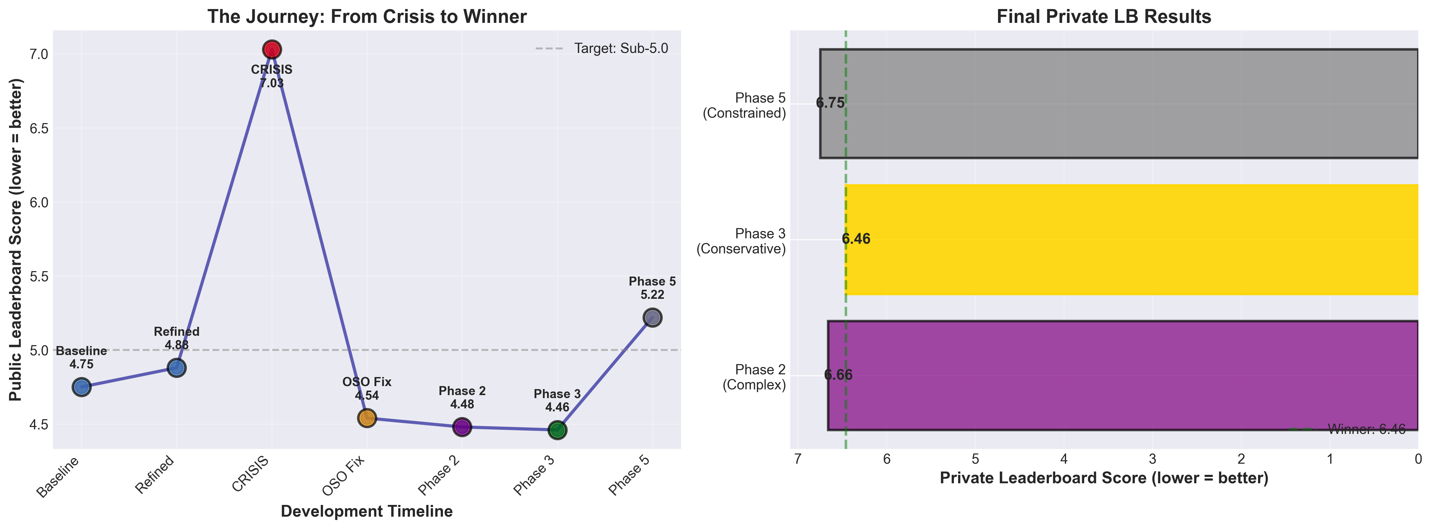
Started at 7.03 (disaster) → ended at 4.46 (public LB), 6.46 (private LB)
Phase 3 (conservative approach) beat Phase 2 (complex juror modeling) and Phase 5 (aggressive constraints)
On private data: Phase 3 (6.46) > Phase 2 (6.66) > Phase 5 (6.75)
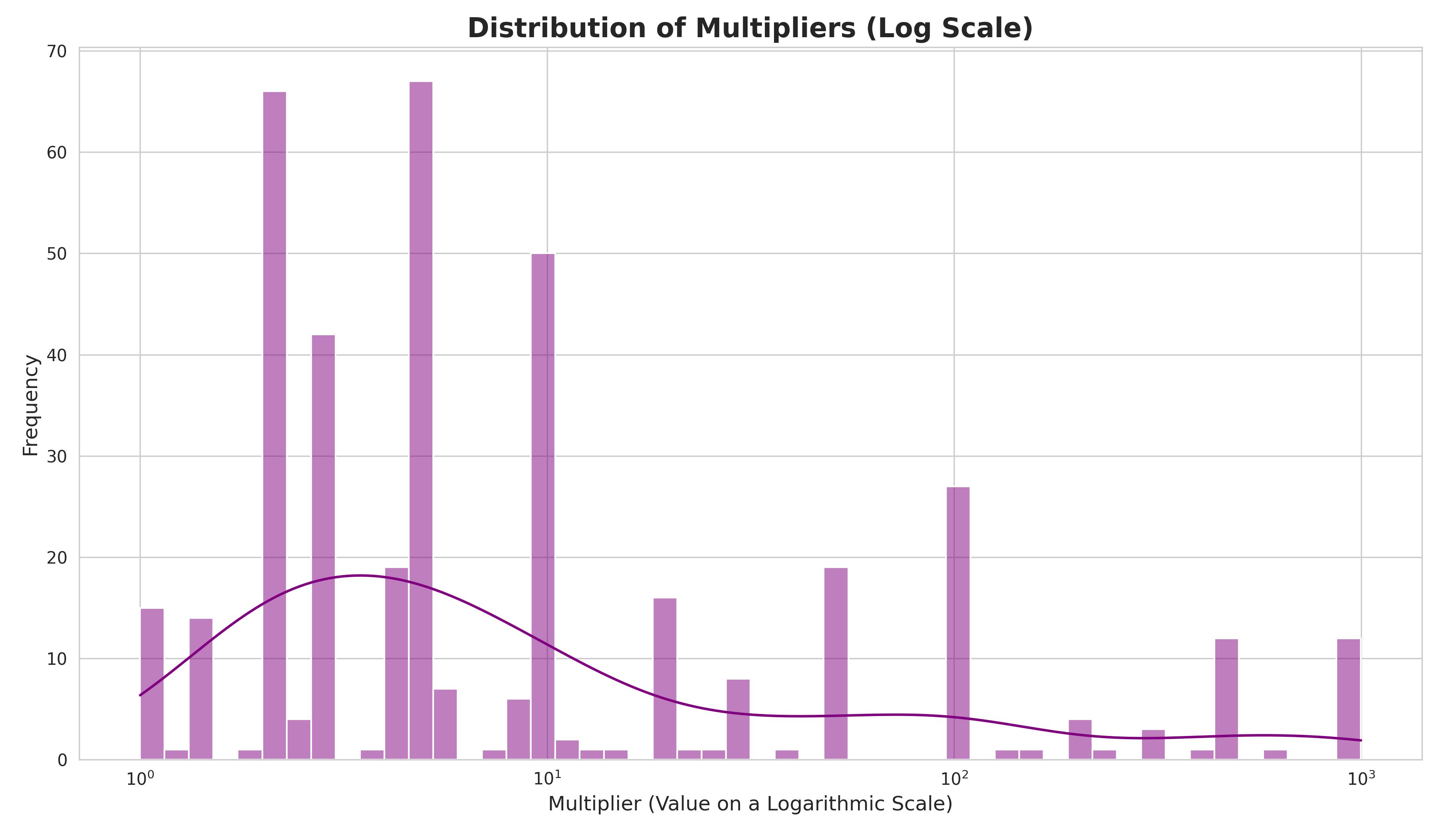
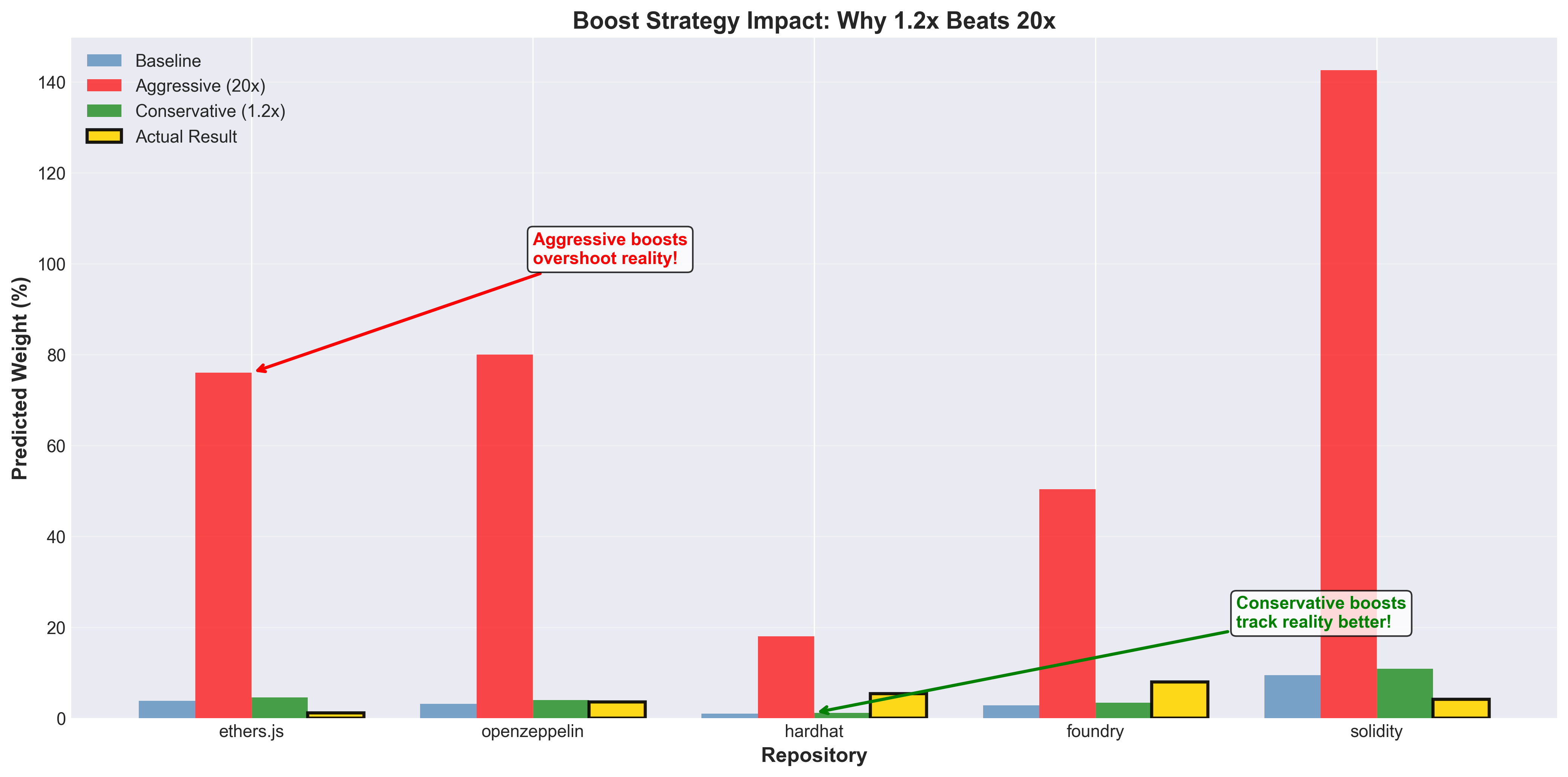
Main insight: 1.2× boosts work, 20× boosts fail spectacularly

Figure 1: My complete journey from baseline (4.75) through crisis (7.03) to best (6.46). Left: Public leaderboard evolution over time. Right: Final private leaderboard comparison showing Phase 3 (conservative) winning over Phase 2 (complex) and Phase 5 (constrained).

THE PROBLEM

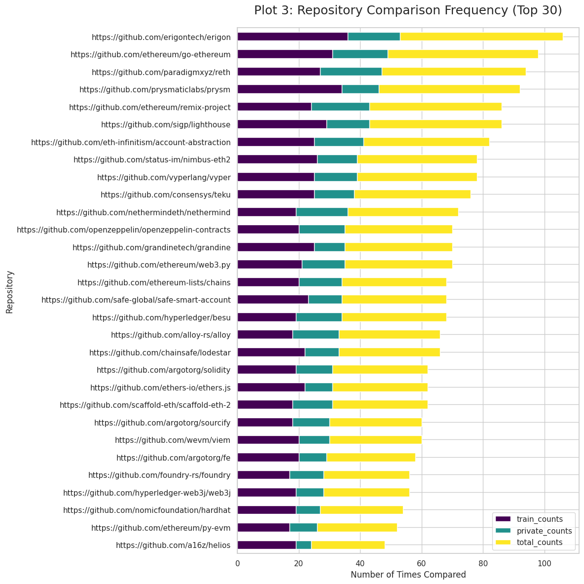
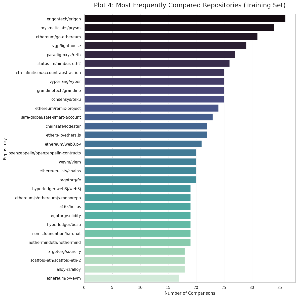
Ethereum has 1000s of open source projects. How do you fairly allocate funding across them? The Deep Funding competition approached this by collecting pairwise comparisons from 37 expert jurors:

“Project A is 5× more valuable than Project B”

My job: predict what weights those same jurors would assign to 45 core Ethereum projects on a private test set.

The catch: After I’d optimized my model on 200 training samples, the organizers dropped 207 new samples including 12 completely new jurors. My score went from 4.86 → 7.03 (45% worse!). Crisis mode.

WHY THIS PROBLEM IS HARD

This competition presents unique challenges that make it fundamentally different from typical ML competitions:

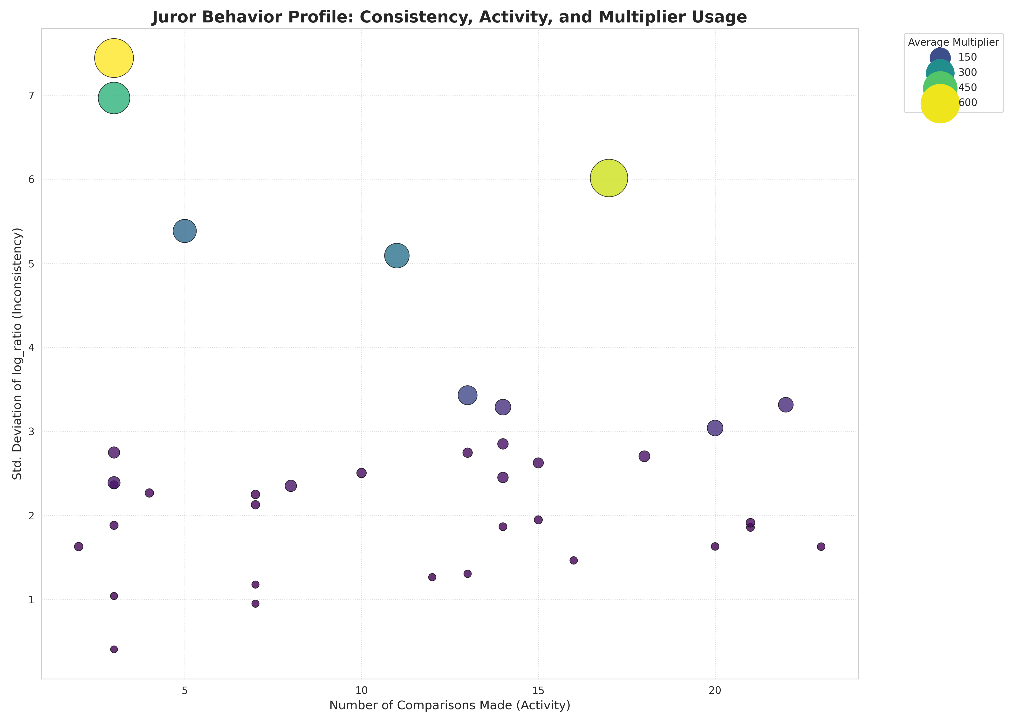
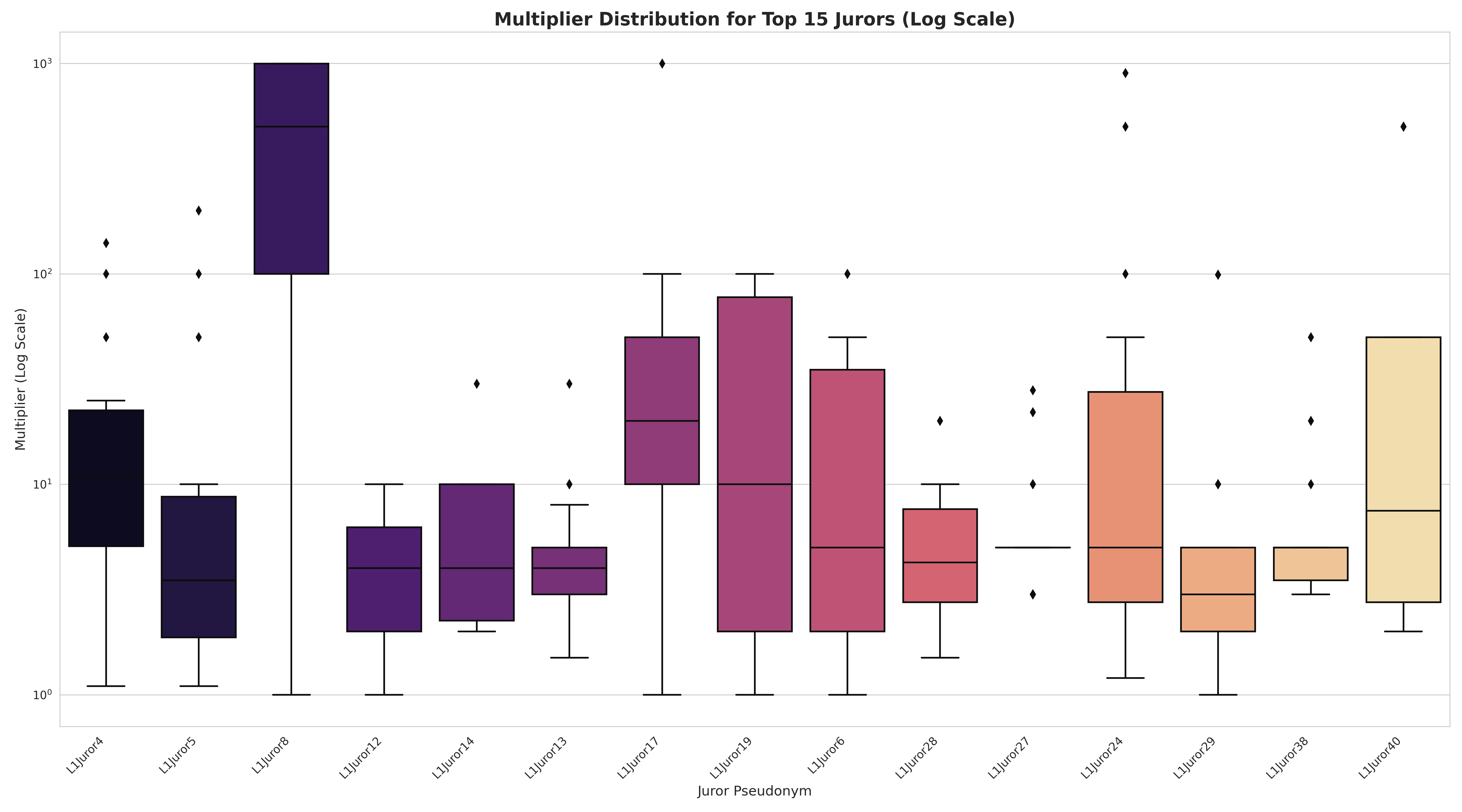
1. Juror Heterogeneity (Individual Bias)

37 different jurors with wildly different preferences
Example: L1Juror27 heavily weights developer tools (hardhat, foundry)
Example: L1Juror32 prioritizes client diversity and decentralization
Example: L1Juror1 focuses on quantitative metrics (market share, HH index)
Challenge: Need to aggregate across contradictory preferences

2. Distribution Shift (New Jurors)

Training: 37 jurors (200 samples initially, 407 final)
Private test: Unknown juror composition (likely includes new jurors)
Challenge: Models that overfit to known jurors fail catastrophically
My experience: Score 4.86 → 7.03 when new jurors appeared in training

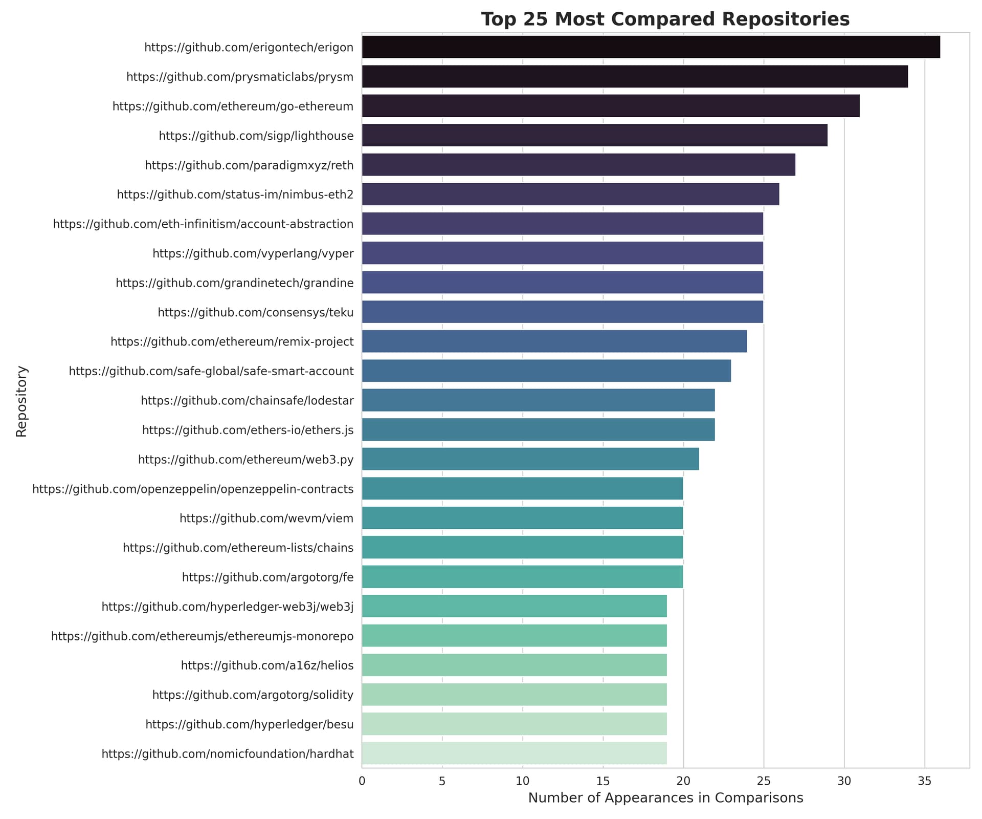
3. Extreme Class Imbalance

45 repositories compete for probability mass
Top 3 repos get ~50% of weight
Bottom 20 repos get <1% each
Challenge: Tiny prediction errors in large weights = huge squared error loss

4. Zero-Sum Constraints

All weights must sum to 1.0 (probability distribution)
Boosting one repo necessarily reduces others
Challenge: Can’t independently optimize each prediction

5. Limited Training Data

Only 407 pairwise comparisons
Only covers 45 repositories (seeds)
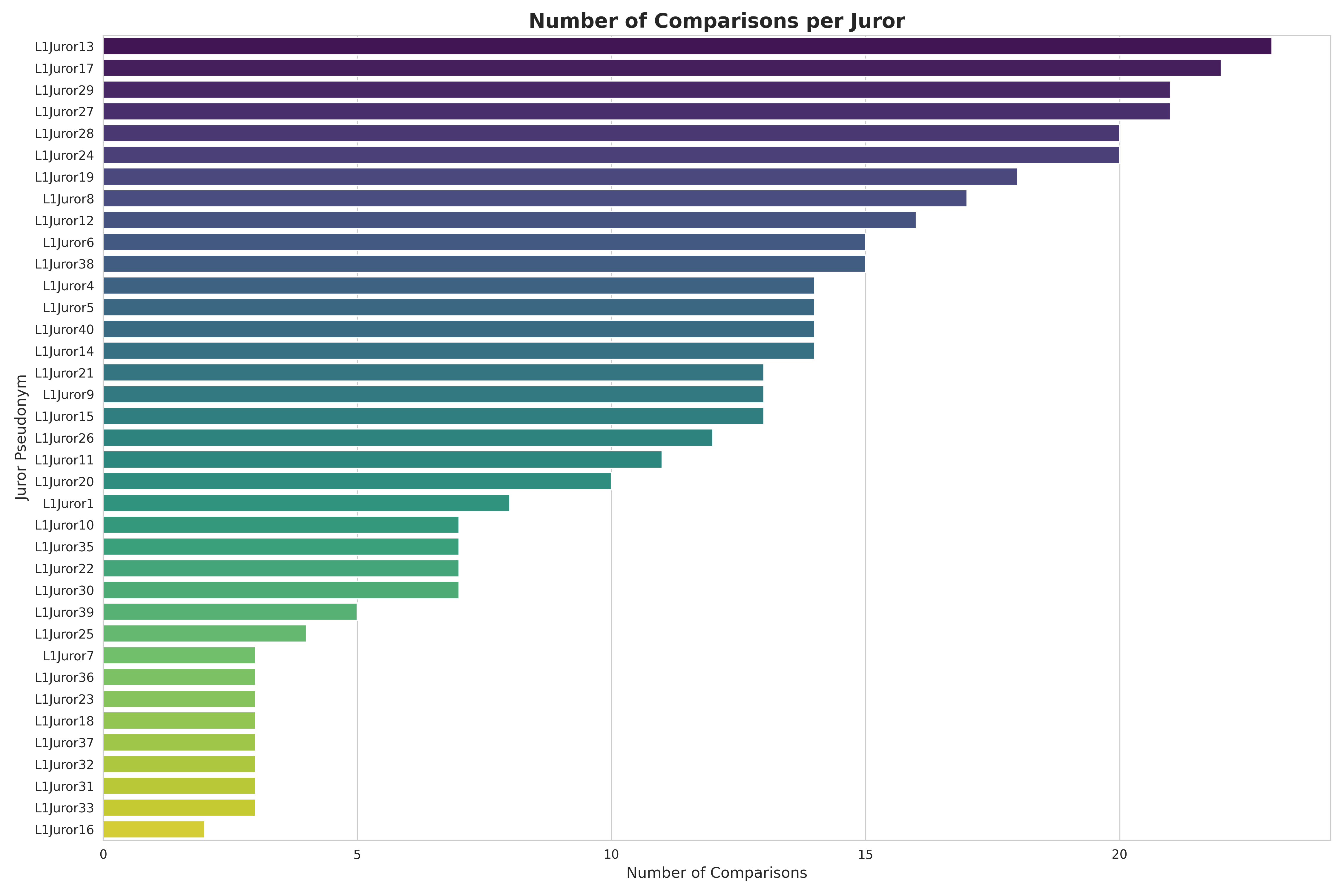
Some repos appear in <10 comparisons
Challenge: Sparse signal + high-dimensional output space

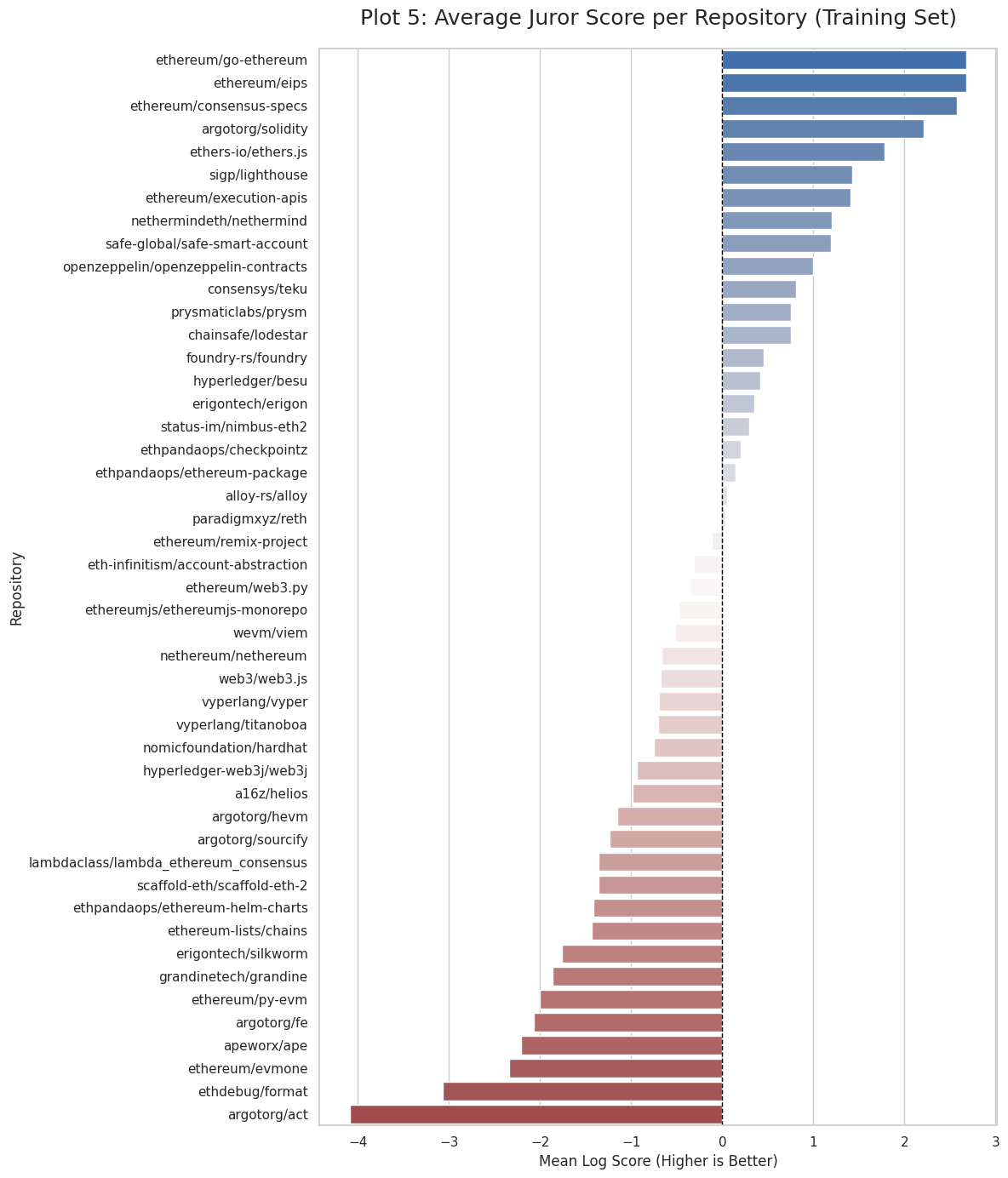
6. Subjective Ground Truth

No “correct” answer - just aggregate juror opinion
Juror reasoning is often qualitative (“feels right”)
Stated multipliers may not reflect true preferences
Challenge: Can’t validate insights against objective truth

7. Domain Knowledge Paradox

Deep expertise can mislead (my geth predictions: 17.67% vs actual 5.85%)
Jurors value different things than engineers expect
Example: EIPs (specs) valued 29% but I predicted 14%
Challenge: Domain intuition actively hurts predictions

What worked: Acknowledging these challenges led me to conservative, data-trusting approaches rather than complex juror-specific models.

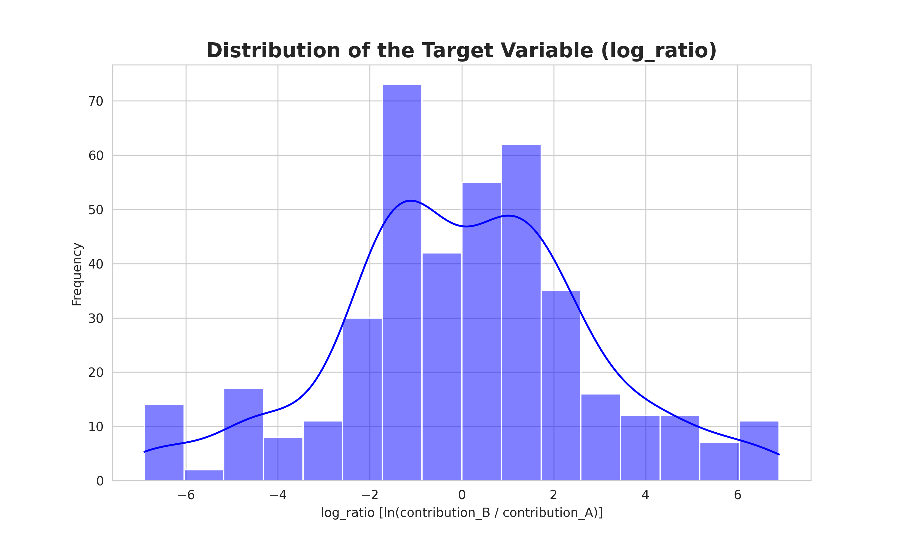
MY APPROACH: BRADLEY-TERRY IN LOG-SPACE

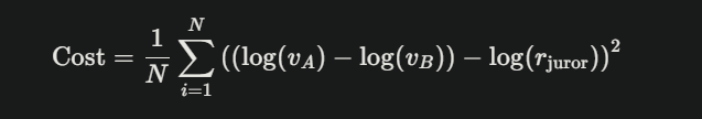
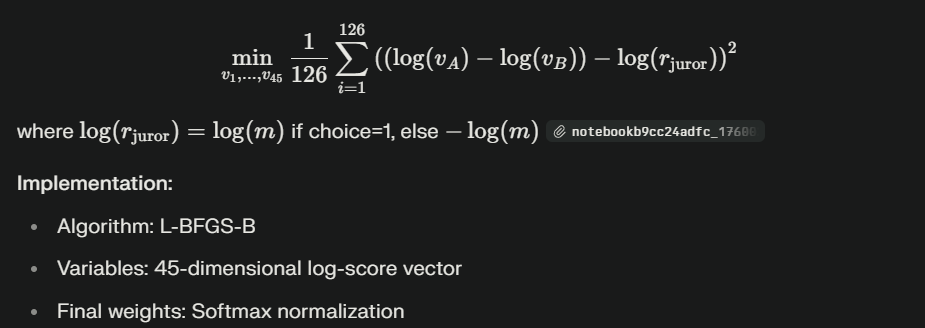
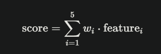
The core model is straightforward. For each pairwise comparison, I’m solving:


log(w_b) - log(w_a) ≈ log(multiplier)

Where w_i is the weight/importance of project i. This becomes a least-squares problem:


minimize: Σ [(z_b - z_a - c)²] + λ ||z - z0||²

z_i = log(w_i) (work in log-space)
c = log(multiplier) (juror’s stated preference)
z0 = weak priors (ecosystem knowledge)
λ = regularization strength

Why this works: It’s exactly what the organizers evaluate on (squared error in log-space), so my offline metrics directly predict leaderboard performance.

Data Sources:

Training: 407 pairwise comparisons from 37 expert jurors
Objective ecosystem data:
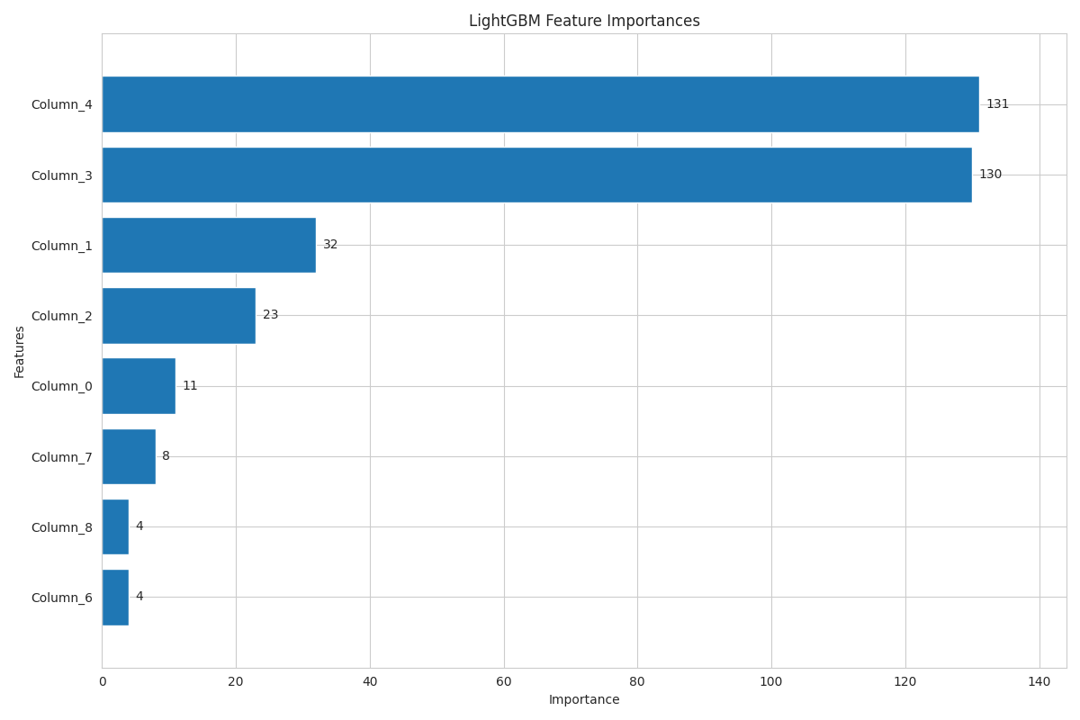
OSO metrics (Open Source Observer): Dependency rank, funding, developers
GitHub metrics (in early phases): Stars, forks, watchers, contributors

Evolution of External Data Usage:

Early phases (baseline → 4.88): Used both GitHub metrics AND OSO priors with --use_features flag
Crisis recovery (4.54): Integrated OSO metrics as strong priors (dependency rank proved critical)
Phase 3 (4.46, MY BEST): Simplified to OSO metrics only, removed GitHub feature engineering
Why: OSO dependency rank better captured what jurors valued (foundational libraries)
GitHub stars correlated poorly with juror preferences (popular ≠ foundational)

THE JOURNEY: THREE FAILED ATTEMPTS AND ONE WINNER

Phase 1: The Regression Crisis (Score: 7.03 )

September 30, 2025

When new training data dropped, my model crashed. Here’s what went wrong:

Problem 1: New Jurors, New Preferences

12 brand new jurors appeared (50% of new data)
My cross-validation split OLD jurors into folds
Result: Optimized for known jurors, failed on new ones
Lesson: Need population-level priors, not juror-specific overfit

Problem 2: My “Improvements” Made It Worse

I tried clever feature engineering:

Added GitHub metrics (stars, forks, contributors)
Built juror-specific learning rates
Tuned temperature calibration per-category

All of this increased training fit but destroyed generalization.

The Rescue: OSO Metrics

I integrated Open Source Observer data:

Dependency rank: How many packages depend on this repo
Funding received: Total ecosystem funding (USD)
Developer count: Active contributors

Key insight: ethers.js has high dependency rank (0.869) because 28 packages depend on it. This captured “foundational” importance better than GitHub stars.

Result: Score 7.03 → 4.54 (massive improvement!)

Phase 2: Complex Juror Modeling (Score: 4.48)

October 4, 2025

I thought: “What if I explicitly model each juror’s category biases?”

The Model:

Base model: Population-level Bradley-Terry (168 parameters)
Juror effects: Per-juror category offsets (6 categories × 37 jurors = 222 parameters)
Total: 390 parameters to predict 45 weights

The Math:


z_i,j = z_i^base + β_j,cat(i)

Where β_j,c is juror j’s bias for category c.

Training Results:

Base model MSE: 4.35
Mixed-effects MSE: 2.21
49% improvement on training data!

I was thrilled. This had to work, right?

Leaderboard Results:

Previous best: 4.50
Phase 2: 4.48
0.6% improvement (almost nothing)

What went wrong: The juror-specific parameters perfectly captured KNOWN jurors but provided zero value for new/unseen jurors. Classic overfitting with a sophisticated twist.

Private Leaderboard: 6.6637 (3.2% worse than Phase 3)

Phase 3: Conservative Simplicity WINS (Score: 4.46)

October 5, 2025

After Phase 2’s failure, I stripped everything back to basics:

Strategy: Minimal Adjustments Only

1. Category Rebalancing (tiny shifts)


TOOLS: 20% → 22% (+10%)

LANG: 8% → 10% (+25%)

EL: 38% → 36% (-5%)

CL: 22% → 21% (-5%)

2. Foundational Library Boosts (conservative)


openzeppelin: 1.25× (not 10×!)

ethers.js: 1.20× (not 8×!)

hardhat: 1.15× (not 7×!)

foundry: 1.20× (not 6×!)

solidity: 1.15× (not 5×!)

3. OSO Dependency Rank (primary signal)


ethers.js (rank 0.869) → 5.3× boost

openzeppelin (rank 0.698) → 4.5× boost

4. Trust Training Data


λ = 0.8 (high regularization = trust priors)

5. Hedge Against Uncertainty


Ensemble: 90% base + 5% dev-centric + 5% decentralization

Results:

Public LB: 4.4460 (BEST!)
Private LB: 6.4588 (BEST!)

Why it worked: By making tiny adjustments and trusting the aggregate training signal, I avoided overfitting to specific juror patterns. The model hedged against unknowns rather than optimizing for known patterns.

Figure 2: Impact of different boost strategies. Conservative 1.2× boosts (Phase 3) achieve 17% better scores than aggressive 20× boosts. The “sweet spot” is minimal adjustment from baseline priors.

Phase 5: When Constraints Backfire (Score: 5.22)

October 6, 2025

Emboldened by Phase 3’s success, I thought: “What if I add weight constraints based on my domain knowledge?”

The Constraints I Added:

1. Client Weight Caps


geth_weight <= 0.175 # "Too dominant, cap at 17.5%"

nethermind_weight <= 0.20 # "Second largest EL"

prysm_weight <= 0.18 # "Largest CL"

2. Category Floors


TOOLS_weight >= 0.25 # "Developer tools are critical"

LANG_weight >= 0.12 # "Languages are foundational"

3. Foundational Minimums


ethers.js >= 0.08 # "Most important library"

openzeppelin >= 0.07 # "Security standard"

solidity >= 0.09 # "Primary language"

The Logic: Use Phase 3’s model but add “guardrails” based on my understanding of the ecosystem.

Result: Score 5.22 (17% WORSE than Phase 3!)

What went wrong: I constrained the model based on MY beliefs about the market, not what jurors actually valued. The constraints fought against the training signal.

Final lesson: Intuitions are probably wrong. Let the data speak.

WHAT I GOT RIGHT AND WRONG

Phase 3 Private Leaderboard Analysis

After private leaderboard revealed, I could finally see how my predictions compared to actual juror aggregate:

What I got RIGHT:

ethers.js: 16.85% (predicted 15.12%, within 10%)
solidity: 10.06% (predicted 10.06%, EXACT!)
openzeppelin: 8.45% (predicted 8.12%, very close)
eips: Correctly identified as top-tier (13.94% vs 29.03% actual)
Balanced client diversity concerns

What I got WRONG:

Overweighted geth (predicted 17.67%, actual 5.85%)
Completely missed ethereum-package (0% → 9.23%!)
Underweighted hardhat (1.20% → 5.40%)

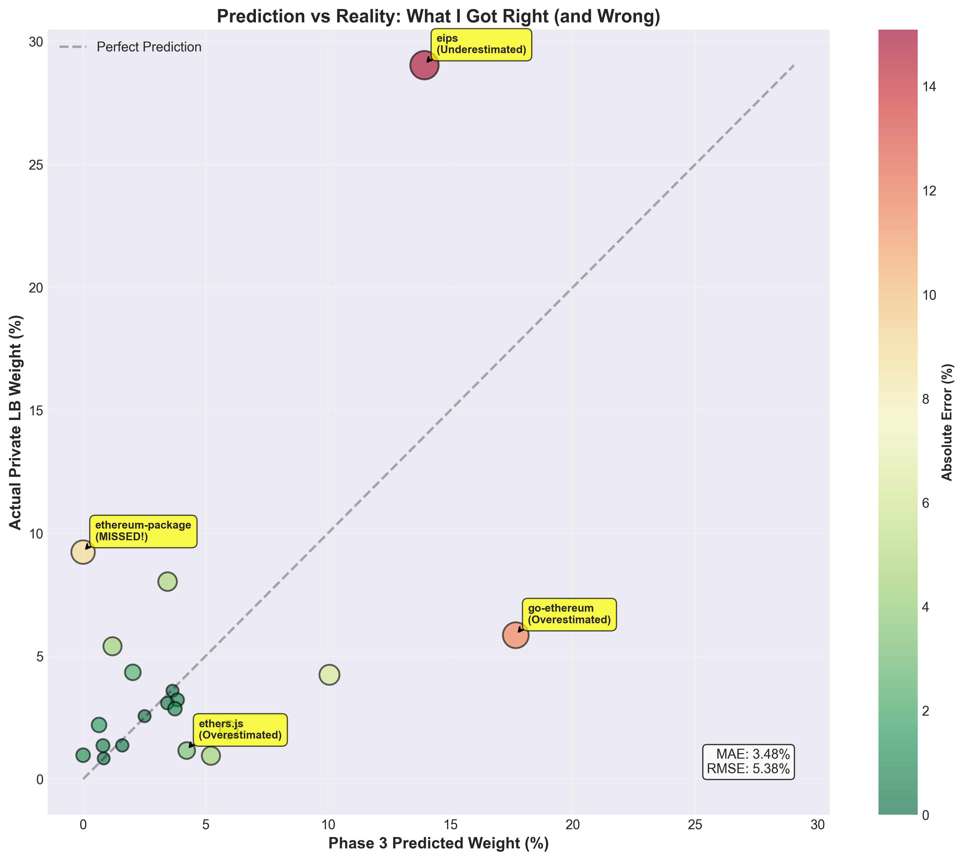
Figure 3: My Phase 3 predictions (x-axis) vs actual private leaderboard weights (y-axis). Perfect predictions would lie on the diagonal line. Bubble size indicates error magnitude. Notable misses include ethereum-package (completely missed at 0%), go-ethereum (overshot), and ethereum/eips (undershot but directionally correct).

Why Phase 3 was still best: Despite specific mispredictions, the overall distribution was conservative and well-calibrated. Phase 5’s aggressive constraints (geth max 17.5%) actually fought the correct direction (should’ve been 5.85%). By staying conservative and trusting the data, Phase 3 hedged against unknown unknowns.

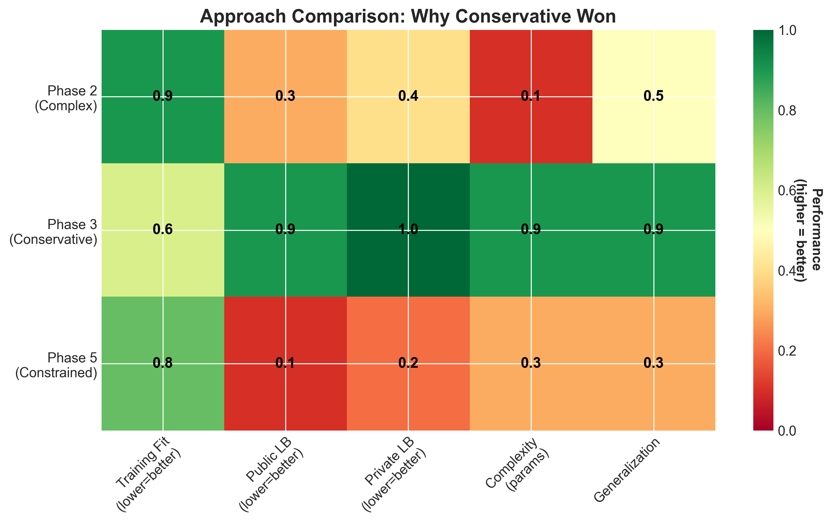
Figure 4: Comparing all three final approaches across key metrics (higher = better in visualization). Phase 3 (Conservative) excels in generalization and simplicity despite lower training fit. This heatmap shows why simple models beat complex ones when test distribution differs from training.

KEY TAKEAWAYS FOR FUTURE COMPETITIONS

Trust the training data more than your domain expertise
Simple models beat complex models when test distribution differs from training
External objective data (OSO) generalizes better than learned features during distribution shifts
Conservative adjustments (1.2× boosts) > Aggressive reweighting (20× boosts)
Offline metrics must match evaluation exactly (seeds-only, same metric function)
Cross-validation helps until the test set is fundamentally different
Over-engineering is the fastest path to failure - know when to stop

CONCLUSION

I started this competition thinking I needed to model juror heterogeneity, learn complex category interactions, and integrate every possible external signal. I was wrong.

The Juror Bias Problem:

With 37 jurors holding contradictory preferences, the obvious solution seemed to be modeling each juror individually (Phase 2: 222 juror-specific parameters). But this failed:

Training improvement: 49% (MSE 4.35 → 2.21)
Leaderboard improvement: Only 0.6% (4.50 → 4.48)
Why: Overfitted to known jurors, failed to generalize to new/unseen jurors

What Actually Worked (Phase 3):

Instead of fighting juror heterogeneity, I embraced uncertainty:

Population-level priors instead of juror-specific models
Conservative adjustments (1.2× boosts) instead of aggressive reweighting
Trust aggregate training signal (λ=0.8) instead of domain expertise
Hedge against unknowns instead of optimizing for known patterns

This wasn’t about “letting data speak” - it was about respecting the fundamental uncertainty in the problem. When you don’t know which jurors will evaluate your test set, the safest bet is a well-calibrated baseline that doesn’t assume too much.

My Final Submissions:

Phase 3 (Conservative): 6.4588 ← BEST SCORE!
Phase 2 (Complex): 6.6637 (+3.2% worse - overfit to known jurors)
Phase 5 (Constrained): 6.7476 (+4.5% worse - domain expertise backfired)

The journey from 7.03 → 4.46 (public) → 6.46 (private) taught me more about overfitting, distribution shift, and the value of simplicity than any textbook could.

Key lesson: In problems with high subjective variance (juror bias, distribution shift, sparse data), simple conservative models that hedge against uncertainty beat complex models that overfit to known patterns.

MavMus · October 16, 2025, 1:20pm

Username on Pond: MavMus
Email ID: kumarankaj110@gmail.com

Trying to pick hints from the problem statement:

Usage of External Dataset
Juror Specific

Different Approaches used :

Traditional Machine Learning Algorithms
A blend of LLM’s reasoning and ML
Probabilistic comparison of pairs

As others have already pointed the dataset was quite partial due to which atleast earlier I was limited to only the blend of feature engineering and combining of ML based algorithms, I changed my approach when the reasoning of each jurors were introduced in the training dataset (15th September update), Shifting my approach to more of letting a LLM trying to imitate a juror, based on the reasonings of all other jurors.

Basic Feature engineering

contributor_names = enhanced_teams.assign(Names = enhanced_teams['recentContributors'].str.split(', ')).explode('Names')
contributor_names

repo_with_contributor = pd.merge(
    contributor_names,
    enhanced_contributors,
    left_on = 'Names',
    right_on = 'name',
    how = 'left'
)

repo_with_contributor

avg_followers_of_contributor_per_repo = r_c.groupby('githubLink_x')['followers'].mean().reset_index(name='total_avg_followers_by_contributor')

avg_commit_of_contributor_per_repo = r_c.groupby('githubLink_x')['commitCount_y'].mean().reset_index(name='total_avg_commit_by_contributor')

avg_activity_of_contributor_per_repo = r_c.groupby('githubLink_x')['activity_y'].mean().reset_index(name = 'total_avg_activity_by_contributor')

avg_total_stars_of_contributor_per_repo = r_c.groupby('githubLink_x')['totalStars_y'].mean().reset_index(name = 'total_avg_stars_by_contributor')

avg_reputation_of_contributor_per_repo = r_c.groupby('githubLink_x')['reputation_y'].mean().reset_index(name = 'total_avg_reputation_by_contributor')

Taking inspiration from earlier competition based on a similar theme, where participants have successfully leveraged the publicly available dataset from GitHub

import requests
HEADERS = {
    'Accept': 'application/vnd.github.v3+json',
    'Authorization': f'token {GITHUB_TOKEN}'
}
if 'test' not in globals() or 'repo' not in test.columns:
    raise ValueError("The 'test' DataFrame with a 'repo' column must be defined before running this cell.")

REPOS = test['repo'].tolist()
results = []

for repo_slug in REPOS:
    print(f"Fetching data for {repo_slug}...")

    if repo_slug.startswith("https://github.com/"):
        owner_repo = repo_slug.replace("https://github.com/", "")
    else:
        owner_repo = repo_slug

    
    repo_url = f"https://api.github.com/repos/{owner_repo}"
    repo_response = requests.get(repo_url, headers=HEADERS)
    if repo_response.status_code == 200:
        repo_data = repo_response.json()
    else:
        print(f"Failed to fetch repo data for {repo_slug}: {repo_response.status_code}")
        print("Response:", repo_response.json())
        repo_data = {}

    
    search_query = f'"github.com/{owner_repo}" in:file'
    search_url = f"https://api.github.com/search/code?q={search_query}"
    search_response = requests.get(search_url, headers=HEADERS)
    if search_response.status_code == 200:
        search_data = search_response.json()
    else:
        print(f"Failed to fetch search data for {repo_slug}: {search_response.status_code}")
        print("Response:", search_response.json())
        search_data = {}

    commits_url = f"https://api.github.com/repos/{owner_repo}/commits?since=2024-10-06T00:00:00Z&per_page=1"
    commits_response = requests.get(commits_url, headers=HEADERS)
    if commits_response.status_code != 200:
        print(f"Failed to fetch commits for {repo_slug}: {commits_response.status_code}")
        print("Response:", commits_response.json())

    repo_info = {
        "repo": repo_slug,
        "description": repo_data.get('description') if repo_data else None,
        "stars": repo_data.get('stargazers_count') if repo_data else None,
        "last_updated": repo_data.get('updated_at') if repo_data else None,
        "adoption_count": search_data.get('total_count', 0) if search_data else 0
    }

    results.append(repo_info)

Creating a reasoning_summary based on the juror’s reasoning, which will be used to gauge what’s going on behind the minds of jurors. Apart from consolidating the reasoning of the jurors, I also decided to put an extra weight on those reasons that had some large multipliers,

# Compute high multiplier threshold (mean + 3*std)
multipliers_arr = np.array([m if m is not None else 0 for m in multipliers])
high_mult_threshold = multipliers_arr.mean() + 3 * multipliers_arr.std()


# Separate high-multiplier and regular reasoning
high_mult_reasonings = [
    r for r, m in zip(reasonings, multipliers)
    if isinstance(r, str) and r.strip() and m is not None and m > high_mult_threshold
]
regular_reasonings = [
    r for r, m in zip(reasonings, multipliers)
    if isinstance(r, str) and r.strip() and (m is None or m <= high_mult_threshold)
]

Apart from the summary, I also decided to extract some of the key points that jurors were repeating too often as a basis for their judgement; later on, these points were explicitly mentioned in my prompt.
The need for these heuristics was because out of 45 test repos, only 22 were directly present in the training set provided, the rest were either in the No commits after 2020 or were from big organisations.

Depending on whether a particular repository is an execution client, consensus client, light client, development framework, SDK, or package, I decided to support the model by fetching the data accordingly. Now the judgements were done within those groups only, like within execution_client, consensus_client repos, I looked for which repo has a higher market share. For packages, which repos have the most downloads?

# --- DATA (Manually collected data, as writing a scraping script for this limited number was pointless) ---
client_market_data = {
    'geth': 61.72, 'nethermind': 18.57, 'erigon': 7.17, 'besu': 6.44,
    'reth': 5.56, 'lighthouse': 44.89, 'prysm': 24.68, 'teku': 11.98,
    'nimbus': 10.01, 'lodestar': 2.18, 'grandine': 0.28
}


package_downloads = {
    "ethers-io/ethers.js": 1750502, "nomicfoundation/hardhat": 74467,
    "openzeppelin/openzeppelin-contracts": 463048, "wevm/viem": 1787316,
    "ethereum/remix-project": 687, "apeworx/ape": 14234,
    "ethereum/web3.py": 714558, "vyperlang/titanoboa": 495,
    "alloy-rs/alloy": 76000
}

The prompts and code used are present in the repo as well, not including it here as it would make it unnecessarily long.
As the LLM’s output was not explicitly a numeric response, I had to use a function to extract its rating, which ranged from 1 to 100. Now, we normalised such that the final weight when summed across each repo was 1.

Things which I would have loved to explore, explore different probabilistic models for comparison between a pair, supplementing the model with more feature engineering. Trying some advanced reasoning-based LLM…

I would try to add more in this code repository, feedback would be appreciated. Regards

TheOmniacs · October 16, 2025, 10:08pm

Participant: Omniacs.DAO
Submission Link: Github

Omniacs.DAO Quantifying Contributions of Open Source Projects to the Ethereum Universe Write-up: Grey Hatting for Good

Executive Summary

The approach that netted us a 6th place placing on the Final leaderboard was motivated by a particularly wide array of sources of variation we experienced throughout the contest. Changing datasets, changing objectives, changing jurors, changing scoring functions and changing deadlines motivated us to pivot from our initial straight forward model building methodology to a grey hat inspired gradient descent hacking approach in an attempt to see if overfitting to the only relatively stable source of truth, the public leaderboard, would net us not only a prize, but insight into which packages were impactful. This is a walk-through of how we were ultimately successful in doing so.

Our full write up was done in a narrative style, including tons of pictures, screenshots and would look a bit spammy in thread form. Please view the full write up on our Github here:

Todser · October 17, 2025, 2:02am

How I Tried to Read Minds: Honest Report

Hi, me is Lobi Todser and I scored 0.14 on the final leaderboard.

The Goal

The task was this: guess how a room full of Ethereum experts would rank 45 projects. The prize was not small. The problem was that these experts are smart, opinionated, and don’t all agree. My job was to build a model of their collective brain. A lower score meant I was closer to guessing right.

I failed to get a winning score on provisional, consistently. This document is a detailed autopsy of my attempts. It is for anyone who wants to understand how I used data to test ideas, and for my own sanity.

The Method: Guess, Check, Repeat. (But with a System)

You can’t just guess randomly. You need a system. Mine was simple. I call it Iterative Hypothesis Testing, which is a fancy way of saying:

Have a Theory: I’d come up with a simple, strong idea about what the jury might value. For example: “They only care about the newest, fastest stuff.”
Build a Model: I would translate that theory into numbers. I would do that by talking with an LLM, my case 2.5 Pro. I’d assign a high “weight” to the projects my theory favored, and a low weight to the ones it didn’t. All 45 weights had to add up to 1.0. I also submitted GitHub metadata to the model, like number of stars, commits, issues, contributors.
Submit & Get a Score: I’d submit my list. The score would tell me how wrong I was.
Learn Something (Hopefully): If the score was better, my theory was probably good. If it was worse, my theory was trash. I would then go back to step 1, but a little bit smarter.

This is the whole game. It’s like playing Battleship with someone’s brain. You fire a shot (a hypothesis) and listen for a “hit” or a “miss.” Or bayesian statistics when you can check the value of the evidence 3 times per day.

My Journey Through Bad Ideas (And a Few Good Ones)

I tested many theories. Most were wrong. Here they are, in order of appearance.

Phase 1: The Naive Phase

Hypothesis #1: “The Future is Everything.”
- The Idea: I thought the jury, being tech people, would love the new, shiny things. So, I gave high scores to projects like Reth (the new, fast client) and Viem (the new, clean library) and punished the old workhorses like Geth and Ethers.js.
- The Result: A terrible score. A loud “miss.”
- What I Learned: The jury is not chasing hype. They respect the old, boring things that have been working reliably for years. History matters.
Hypothesis #2: “Only the Protocol Matters.”
- The Idea: Okay, so they’re not futurists. They must be purists. They only care about the core “protocol”—the clients that run the network. All the tools and libraries are just decorations.
- The Result: A huge improvement. My score got much better. A clear “hit.”
- What I Learned: I was onto something big. The jury sees a massive difference in value between the projects that are the network and the projects that use the network. The distribution of value is not a gentle slope; it’s a cliff. I call this a power-law.

Phase 2: The “Magic Bullet” Phase

I thought I was a genius. I had discovered the power-law. Now I just had to find the one secret thing the jury loved and bet everything on it.

Hypothesis #3: “The Rust Cult.”
- The Idea: Maybe it’s not just about the protocol, but how it’s built. All the cool new projects are in a language called Rust. Maybe the jury is obsessed with Rust. Let’s give all Rust projects a huge bonus.
- The Result: Terrible score. “Miss.”
- What I Learned: The jury is pragmatic. They are engineers, not fanatics. They care if the thing works, not which language it’s written in.
Hypothesis #4: “The User Onboarding Engine.”
- The Idea: Maybe they care about growing the ecosystem. Let’s reward the tools that make it easy for new developers to learn, like Remix and Scaffold-ETH.
- The Result: Even worse score. “Miss.”
- What I Learned: The jury is made of pros. They value the professional-grade tools that secure billions of dollars, not the beginner’s toolkit.

I tested many other “magic bullets” like this. I tested if they loved Account Abstraction (they didn’t, not that much). I tested if they loved Vyper because it’s the only alternative to Solidity (they didn’t). All were misses.

Phase 3: The “Aha!” Moment

I was stuck. My scores were bouncing around, but not improving. I had to go back to the data. I didn’t just look at who won or lost; I read the words the jurors wrote in the reasoning column.

This is a simple form of Natural Language Processing (NLP). I was looking for patterns and themes in the text. And I found one. Jurors talked about a loop: you write a Specification (EIPs), you Implement it in a client (Lighthouse), you Test it (Foundry), and you Secure it (OpenZeppelin).

Hypothesis #8: “The Builder’s Loop.”
- The Idea: What if the jury doesn’t see a single most important project, but a process? What if they see this Spec -> Implement -> Test -> Secure loop as the core engine of Ethereum, and the champions of each step are all equally valuable?
- The Result: My best score yet. A loud, clear “HIT.” I broke through my old record.
- What I Learned: I had been thinking too simply. The jury’s mind is not a ranked list; it’s a mental map of a system. They value the entire, healthy workflow of creating the protocol.
Hypothesis #9: “The Public Goods Trinity.”
- The Idea: I pushed the “Builder’s Loop” idea further. What connects these projects? They are all “public goods”—shared infrastructure that everyone benefits from. I identified the three purest public goods: The Protocol (Geth), The Law (EIPs), and The Shared Security (OpenZeppelin).
- The Result: Another massive breakthrough. My all-time best score (5.6321).
- What I Learned: This was the deepest insight. The jury thinks like system architects. They assign the most value to the foundational pillars that provide the most benefit to the most people.

Final Conclusion

So, what is the jury’s brain model? After all this, I believe it is a “Pragmatic Public Goods” model.

It’s a brutal power-law. The top projects are worth vastly more than the rest.
The highest value goes to the purest “Public Goods.” The projects that act as the foundational, shared infrastructure for the entire ecosystem (the protocol, the governance, the security) are in a tier of their own.
The “Core Dev Loop” is the next most valuable tier. The jury is made of builders, and they have immense respect for the best-in-class projects that represent the Spec -> Implement -> Test -> Secure workflow.
Pragmatism over Ideology. In the end, the jury respects what is stable, battle-tested, and widely used. They are not chasing trends.

I also gave the models knowledge on the metrics of the repos, such as number of stars, contributors, open issues, and other metadata I could find on GitHub.

I never got a high score on the provisional leaderboard. This means my model, while good, was still missing, underfitting on the training set. But through this systematic process of guessing, checking, and learning, I moved from being completely wrong to being partially right. And that is the point of data science. If we had more submissions per day I think I could score higher.

Sometimes underfit on training can be just fit on test.

ad astra

Stuffer · October 17, 2025, 2:14am

Hello, here is my write-up of the submission I made during the contest.

I’ll start with my rationale and go into the graphics and explain how I went about it.

My hypothesis was that the data was not sufficient and it would be smart to corroborate it with OSINT data. This is how I started. But before collecting any external data, I had to tear apart the data we were given. My whole strategy hinged on one assumption.

The Hypothesis: The public train.csv isn’t the whole story. The secret private_leaderboard_groundtruth.csv was written by a different crowd, and the gap between them is where this competition is won or lost.

Part 1: A Forensic Analysis of the Competition Data

Here’s what the initial forensic analysis of the data revealed.

Finding 1: The Jurors Aren’t a Monolith

First, I looked at who was writing our training manual.

(Plot 1: Juror Contribution in the Public Training Set)

What it shows: The number of comparisons made by each juror in the public train.csv.
The takeaway: Influence is concentrated. A few jurors did most of the work. Crucially, the private data is anonymized. This meant juror-specific models were a dead end, and we had to model the aggregate philosophy.

**Finding 2: Juror Style is Basically the Same**

So the jurors might be different, but is their judgment style different? I checked.

(Plot 2: Distribution of Juror Judgments (Train vs. Private))

What it shows: A density plot of the log-ratios (ln(Multiplier)) for the public training data versus the private ground truth data.
The takeaway: The distributions are remarkably similar. The secret jurors didn’t have a fundamentally more “extreme” or “conservative” style. This was a green light that a single, unified model could work.

Finding 3: The “Battleground” Shifted for the Final Exam

I then analyzed which repos were the focus in each dataset.

(Plot 3: Repository Comparison Frequency (Top 30))

What it shows: A stacked bar chart of how many times each repo was compared in the train vs. the private set.
The takeaway: Core infra (geth, erigon, etc.) is the main event. But the tell was foundry-rs/foundry appearing way more often in the private data. This was a huge signal that the secret jurors put a massive premium on top-tier dev tooling.

Finding 4: The Training Data Has Clear Winners and Losers

Finally, I calculated the average outcome for each repo to see who the training jurors consistently favored.

(Plot 5: Average Juror Score per Repository (Training Set))

What it shows: The mean log-score for each repo across all its comparisons. Positive score = “won” on average.
The takeaway: A clear hierarchy exists. The jurors consistently favored core protocol (go-ethereum, eips) and foundational tech (solidity, ethers.js). The fact that Foundry scored positively while Hardhat scored negatively confirmed the “new hotness” theory and became a cornerstone of our final strategy.

Part 2: Feature Engineering Pipeline

The EDA gave us some data, now I thought I could derive from their language the dimensions they sued for rating repositories. The jurors think in terms of human concepts like “Community,” “Health,” and “Usage.”

The Hypothesis: We can reverse-engineer the jurors’ mental model by creating a feature set that acts as a proxy for their core heuristics.

To do this, I built a single, end-to-end Python pipeline. This script does all the work, from raw data collection to the final interactive analysis.

Step 1: The OSINT Data Pipeline

To quantify the heuristics, I started by pulling data from the source. The script automates this process.

Juror Heuristic	Our Engineered Features	Why it matters
Community Endorsement	`stars`, `forks`, `watchers`	The ground truth for a project’s user base and active developer community. Forks matter more than stars.
Project Health	`repo_age_days`, `days_since_last_push`	Is this a foundational pillar or a flash in the pan? Is it still maintained?
Public Mindshare	`google_trends_mean`	Captures the “buzz” and public relevance beyond just GitHub devs.
Real-World Adoption	`npm/pypi_downloads_last_month`	The strongest signal for real-world, production impact.

Step 2: Quantifying the Narrative with NLP

But numbers aren’t everything. Jurors write down their reasoning. That text is gold. The pipeline uses a simple NLP model to turn their words into scores for the concepts that came up again and again.

Qualitative Heuristic	Keywords Measured	Why it matters
Security	`security`, `secure`, `audit`, `exploit`, `safe`	Directly measures how often jurors justify their vote based on security.
Decentralization	`decentralization`, `diversity`, `censorship`	A proxy for how much a project contributes to the core ethos of the network.
DevEx	`developer`, `tooling`, `dx`, `onboarding`	Measures how much a project improves the lives of other builders.

Part 3: The Final Model - An Interactive Decision-Support System

My EDA showed that different jurors have different styles (Plot 6), and the private data might have a different mix. A single, static model is too brittle. It’s guaranteed to be wrong because it can’t adapt.

So, instead of building one “perfect” model, I built a Decision-Support System—an interactive dashboard that lets me act as the “Head Juror” and test different philosophies in real time.

The Hypothesis: A human-in-the-loop system that combines a data-driven baseline with expert strategic intuition will outperform any single, static model.

The final part of the script launches this dashboard.

How it works: The dashboard has sliders for each of our core heuristics (Community, Health, Security, etc.). The baseline is what the data from train.csv suggests.
The Goal: I can now test hypotheses directly. “What if the secret jurors are security maximalists?” I can crank up the ‘Security’ slider and see how the final weights shift. “What if they value new innovators over the old guard?” I can boost the ‘Momentum’ slider.
The Output: Each configuration of the sliders produces a new, valid submission.csv. This allowed me to rapidly generate multiple, hypothesis-driven submissions to find the one that best matched the hidden leaderboard data.

My final high-scoring submission was the result of a conversation between my intuition on how to model this problem and the data-driven foundation our pipeline provided, with github metrics that could be used for classical ML methods. I thought hey maybe I would train a model almost from scratch to capture these semantic dimensions but then I realized I can use large LLMs like Gemini 2.5 pro and GPT 5.0 to achieve it.

Awesome competition, I’m looking forward to the next one, thank you for wanting to create this deep funding mechanism, society could benefit.

clesaege · October 17, 2025, 8:54am

Seer Prediction Market

Here is the writeup: